
9.5: Position in an Elliptic Orbit
- Page ID
- 6845

The reader might like to refer back to Section 2.3, especially the part that deals with the polar Equation to an ellipse, to be reminded of the meanings of the angles \(θ\), \(ω\) and \(v\), which, in an astronomical context, are called, respectively, the argument of latitude, the argument of perihelion and the true anomaly. In this section I shall choose the initial line of polar coordinates to coincide with the major axis of the ellipse, so that \(ω\) is zero and \(θ = v\). The Equation to the ellipse is then
\[r = \frac{l}{1 + e \cos v}. \label{9.6.1} \tag{9.6.1}\]
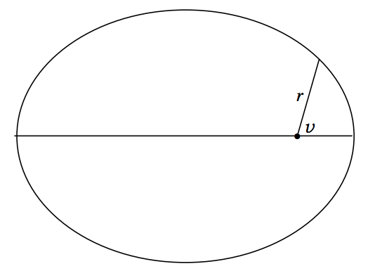
\(\text{FIGURE IX.5}\)
I’ll suppose that a planet is at perihelion at time \(t = T\), and the aim of this section will be to find \(v\) as a function of \(t\). The semi major axis of the ellipse is \(a\), related to the semi latus rectum by
\[l = a (1-e^2) \label{9.6.2} \tag{9.6.2}\]
and the period is given by
\[P^2 = \frac{4 π^2}{G \textbf{M}} a^3. \label{9.6.3} \tag{9.6.3}\]
Here the planet, of mass \(m\) is supposed to be in orbit around the Sun of mass \(M\), and the origin, or pole, of the polar coordinates described by Equation \ref{9.6.1} is the Sun, rather than the centre of mass of the system. As usual, \(\textbf{M} = M + m\).
The radius vector from Sun to planet does not move at constant speed (indeed Kepler’s second law states how it moves), but we can say that, over a complete orbit, it moves at an average angular speed of \(2π/P\). The angle \(\frac{2 π}{P} (t-T)\) is called the mean anomaly of the planet at a time \(t − T\) after perihelion passage. It is generally denoted by the letter \(\text{M}\), which is already overworked in this chapter for various masses and functions of the masses. For mean anomaly, I’ll try this font: \(\mathcal{M}\). Thus
\[\mathcal{M} = \frac{2π}{P} (t-T). \label{9.6.4} \tag{9.6.4}\]
The first step in our effort to find \(v\) as a function of \(t\) is to calculate the eccentric anomaly \(E\) from the mean anomaly. This was defined in figure \(\text{II.11}\) of Chapter 2, and it is reproduced below as figure \(\text{IX.6}\).
In time \(t − T\), the area swept out by the radius vector is the area \(\text{FBP}\), and, because the radius vector sweeps out equal areas in equal times, this area is equal to the fraction \((t −T)/ P\) of the area of the ellipse. In other words, this area is \(\frac{(t-T)π a b}{P}\). Now look at the area \(\text{FBP}^\prime\). Every ordinate of that area is equal to \(a/b\) times the corresponding ordinate of \(\text{FBP}\), and therefore the area of \(\text{FBP}^\prime\) is \(\frac{(t-T) π a^2}{P}\). The area \(\text{FBP}^\prime\) is also equal to the sector \(\text{OP}^\prime \text{B}\) minus the triangle \(\text{OP}^\prime \text{F}\). The area of the sector \(\text{OP}^\prime \text{B}\) is \(\frac{E}{2 π} \times π a^2 = \frac{1}{2} Ea^2\), and the area of the triangle \(\text{OP}^\prime \text{F}\) is \(\frac{1}{2} a e \times a \sin E = \frac{1}{2} a^2 e \sin E\).
\[\therefore \frac{(t-T) π a^2}{P} = \frac{1}{2} E a^2 - \frac{1}{2} a^2 e \sin E.\]
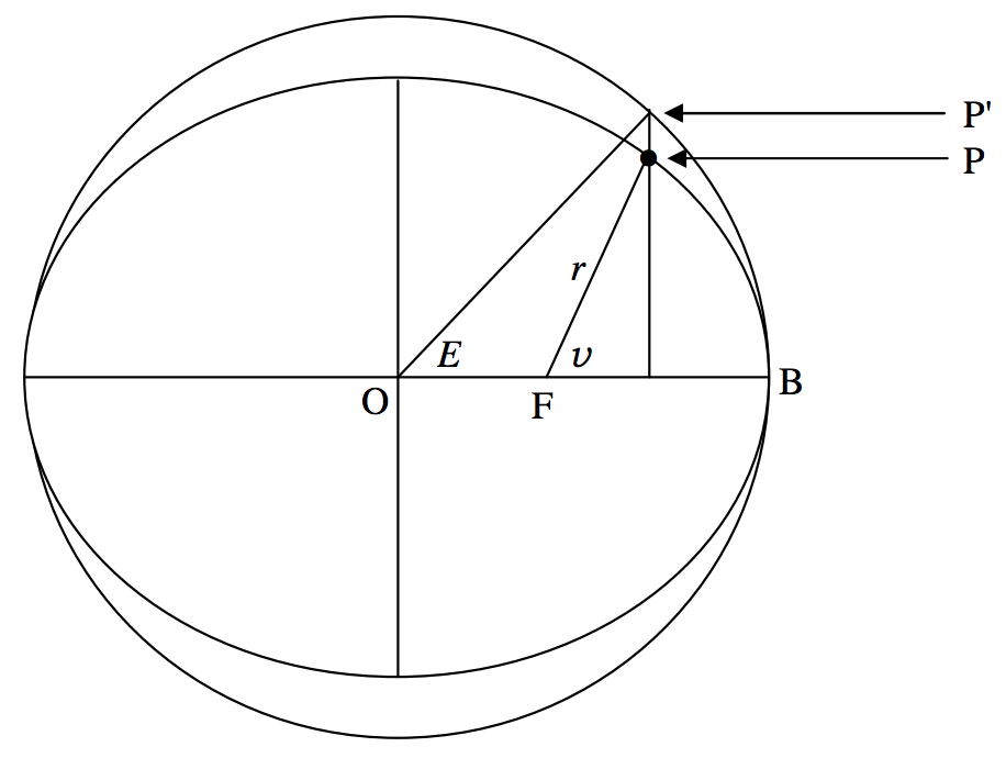
\(\text{FIGURE IX.6}\)
Multiply both sides by \(2/a^2\), and recall Equation \ref{9.6.4}, and we arrive at the required relation between the mean anomaly \(\mathcal{M}\) and the eccentric anomaly \(E\):
\[\mathcal{M} = E - e \sin E . \label{9.6.5} \tag{9.6.5}\]
This is Kepler’s Equation.
The first step, then, is to calculate the mean anomaly \(\mathcal{M}\) from Equation \ref{9.6.4}, and then calculate the eccentric anomaly \(E\) from Equation \ref{9.6.5}. This is a transcendental Equation, so I’ll say a word or two about solving it in a moment, but let’s press on for the time being. We now have to calculate the true anomaly \(v\) from the eccentric anomaly. This is done from the geometry of the ellipse, with no dynamics, and the relation is given in Chapter 2, Equations 2.3.16 and 2.3.17c, which are reproduced here:
\[\cos v = \frac{\cos E - e}{1 - e \cos E}. \label{2.3.16} \tag{2.3.16}\]
From trigonometric identities, this can also be written
\[\sin v = \frac{\sqrt{1- e^2} \sin E}{1-e \cos E}, \label{2.3.17a} \tag{2.3.17a}\]
or \[\tan v = \frac{\sqrt{1 - e^2} \sin E}{\cos E - e} \label{2.3.17b} \tag{2.3.17b}\]
or \[\tan \frac{1}{2} v = \sqrt{\frac{1+e}{1-e}} \tan \frac{1}{2} E. \label{2.3.17c} \tag{2.3.17c}\]
If we can just solve Equation \ref{9.6.5} (Kepler’s Equation), we shall have done what we want – namely, find the true anomaly as a function of the time.
The solution of Kepler’s Equation is in fact very easy. We write it as
\[f(E) = E - e \sin E - \mathcal{M} \label{9.6.6} \tag{9.6.6}\]
from which \[f^\prime (E) = 1 - e \cos E, \label{9.6.7} \tag{9.6.7}\]
and then, by the usual Newton-Raphson process:
\[E = \frac{\mathcal{M} - e(E \cos E - \sin E)}{1- e \cos E}. \label{9.6.8} \tag{9.6.8}\]
The computation is then extraordinarily rapid (especially if you store cos E and don’t calculate it twice!).
Suppose \(e = 0.95\) and that \(M = 245^\circ\). Calculate \(E\). Since the eccentricity is very large, one might expect the convergence to be slow, and also \(E\) is likely to be very different from \(\mathcal{M}\), so it is not easy to make a first guess for \(E\). You might as well try \(245^\circ\) for a first guess for \(E\). You should find that it converges to ten significant figures in a mere four iterations. Even if you make a mindlessly stupid first guess of \(E = 0^\circ\), it converges to ten significant figures in only nine iterations.
There are a few exceptional occasions, hardly ever encountered in practice, and only for eccentricities greater than about \(0.99\), when the Newton-Raphson method will not converge when you make your first guess for \(E\) equal to \(\mathcal{M}\). Charles and Tatum (Celestial Mechanics and Dynamical Astronomy 69, 357 (1998)) have shown that the Newton-Raphson method will always converge if you make your first guess \(E = π\). Nevertheless, the situations where Newton-Raphson will not converge with a first guess of \(E = \mathcal{M}\) are unlikely to be encountered except in almost parabolic orbits, and usually a first guess of \(E = \mathcal{M}\) is faster than a first guess of \(E = π\). Τhe chaotic behaviour of Kepler’s Equation on these exceptional occasions is discussed in the above paper and also by Stumpf (Cel. Mechs. and Dyn. Astron. 74, 95 (1999)) and references therein.
Show that a good first guess for \(E\) is
\[E = \mathcal{M} + x(1 - \frac{1}{2}x^2 ) , \label{9.6.9} \tag{9.6.9}\]
where \[ x = \frac{e \sin \mathcal{M}}{1 - e \cos \mathcal{M}}. \label{9.6.10} \tag{9.6.10}\]
Write a computer program in the language of your choice for solving Kepler’s Equation. The program should accept \(e\) and \(\mathcal{M}\) as input, and return \(E\) as output. The Newton-Raphson iteration should be terminated when \(|(E_{\text{new}} − E_{\text{old}}) / E_{\text{old}}\) is less than some small fraction to be determined by you.
An asteroid is moving in an elliptic orbit of semi major axis \(3 \text{AU}\) and eccentricity 0.6. It is at perihelion at time = 0. Calculate its distance from the Sun and its true anomaly one sidereal year later. You may take the mass of the asteroid and the mass of Earth to be negligible compared with the mass of the Sun. In that case, Equation \ref{9.6.3} is merely
\[P^2 = \frac{4 π^2}{GM}a^3 , \]
where \(M\) is the mass of the Sun, and, if \(P\) is expressed in sidereal years and \(a\) in \(\text{AU}\), this becomes just \(P^2 = a^3\). Thus you can immediately calculate the period in years and hence, from Equation \ref{9.6.4} you can find the mean anomaly. From there, you have to solve Kepler’s Equation to get the eccentric anomaly, and the true anomaly from Equation 2.3.16 or 17. Just make sure that you get the quadrant right.
Write a computer program that will give you the true anomaly and heliocentric distance as a function of time since perihelion passage for an asteroid whose elliptic orbit is characterized by \(a\), \(e\). Run the program for the asteroid of the previous exercise for every day for a complete period.
You are now making some real progress towards ephemeris computation!