16.2: Motion Under a Central Force

There is no general analytical solution in terms of simple algebraic functions for the problem of three gravitating bodies of comparable masses. Except in a few very specific cases the problem has to be solved numerically. However in the restricted three-body problem, we imagine that there are two bodies of comparable masses revolving around their common centre of mass \(\text{C}\), and a third body of negligible mass moves in the field of the other two. We considered this problem partially in Section 16.1, except that we restricted our interest yet further in confining our attention to the line joining to two principal masses. In this section we shall widen our attention. One question that we asked in section 16.1 was: Are there any points where a third body of negligible mass could orbit around \(\text{C}\) with the same period as the other two masses? We found three such points, the collinear lagrangian points, on the line joining the two principal masses. In this section we shall discover two additional points, the fourth and fifth lagrangian points. They are not collinear with \(M_1\) and \(M_2\), but are such that the three masses are at the corners of an equilateral triangle.

We shall work in a co-rotating reference frame in which there are two deep hyperbolic potential wells of the form \(−GM_1 /r_1\) and \(−GM_2 /r_2\) from the gravitational field of the two principal masses sunk into the nose-up paraboloidal potential of the form \(-\frac{1}{2} ρ^2 ω^2\), whose negative derivative is the centrifugal force per unit mass. Here \(ρ\) is the usual cylindrical coordinate, and \(ω^2 = G(M_1 + M_2 ) / a^3 \).

\(\text{FIGURE XVI.7}\)

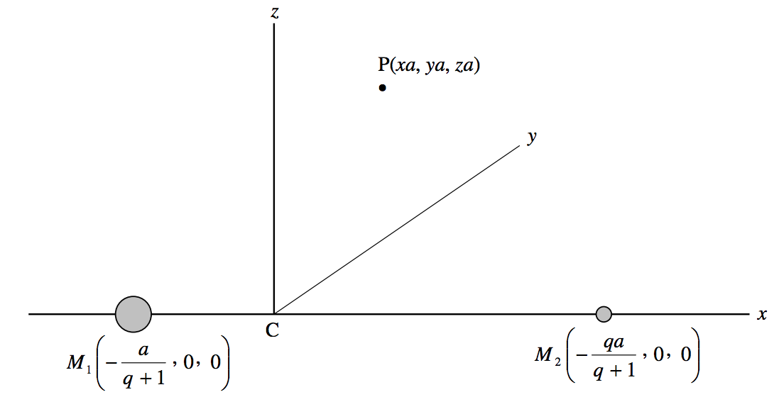
In figure \(\text{XVI.7}\) we see a coordinate system which is rotating about the \(z\)-axis, in such a manner that the two principal masses remain on the x-axis, and the origin of coordinates is the centre of mass \(\text{C}\). The mass ratio \(M_1/M_2 = q\), so the coordinates of the two masses are as shown in the figure. The constant distance between the two masses is \(a\). \(\text{P}\) is a point whose coordinates are \((xa, \ ya , \ za), \ x, \ y\) and \(z\) being dimensionless. The gravitational-plus-centrifugal effective potential \(V\) at \(P\) is

\[V = - \frac{GM_1}{a \left[ \left( x + \frac{1}{q + 1} \right)^2 + y^2 + z^2 \right]^{1/2}} - \frac{GM_2}{a \left[ \left( x - \frac{q}{q + 1} \right)^2 + y^2 + z^2 \right]^{1/2}} - \frac{G(M_1 + M_2)(x^2 + y^2)}{2a}. \label{16.2.1} \tag{16.2.1}\]

Let \(W = \frac{Va}{G(M_1 + M_2)}\) (dimensionless). Then

\[W = - \frac{q}{ \left[ \left( 1 + x (q+1) \right)^2 + (y^2 + z^2 ) (q+1)^2 \right]^{1/2}} - \frac{1}{\left[ \left( q - x(q+1) \right)^2 + (y^2 + z^2)(q+1)^2 \right]^{1/2}} - \frac{x^2 + y^2}{2} . \label{16.2.2} \tag{16.2.2}\]

I shall write this for short:

\[W = -Aq - B - \frac{1}{2} ( x^2 + y^2 ) . \label{16.2.3} \tag{16.2.3}\]

Here \(A\) and \(B\) are functions with obvious meaning from comparison with Equation \ref{16.2.2}.

We are going to need the first and second derivatives, so I list them here, in which, for example, \(W_{xy}\) is short for \(\partial^2 W / \partial x \partial y\).

\[W_x = -(q + 1) [-q \left(1 + x) ( q+1) \right) A^3 + \left( q - x) (q + 1) \right) B^3 ] - x , \label{16.2.4} \tag{16.2.4}\]

\[W_y = (q + 1)^2 y [q A^3 + B^3 ] - y , \label{16.2.5} \tag{16.2.5}\]

\[W_z = (q + 1 )^2 z [q A^3 + B^3], \label{16.2.6} \tag{16.2.6}\]

\[W_{xx} = -(q + 1)^2 [3q \left( 1 + x(q+1) \right)^2 A^5 - qA^3 + 3 \left( q -x (q+1) \right)^2 B^5 - B^3 ] - 1 , \label{16.2.7} \tag{16.2.7}\]

\[W_{yy} = - (q + 1)^2 [3q (q+1)^2 y^2 A^5 - q A^3 + 3 (q+1)^2 y^2 B^5 - B^3] - 1, \label{16.2.8} \tag{16.2.8}\]

\[W_{zz} = -(q + 1)^2 [3q ( q + 1)^2 z^2 A^5 - q A^3 + 3 (q + 1)^2 z^2 B^5 - B^3], \label{16.2.9} \tag{16.2.9}\]

\[W_{yz} = W_{zy} = -3 (q + 1)^4 yz (qA^5 + B^5) , \label{16.2.10} \tag{16.2.10}\]

\[W_{zx} = W_{xz} = -3 ( q+ 1)^3 z [q \left( 1 + x (q + 1) \right) A^5 - \left( q - x(q + 1) \right) B^5 ] , \label{16.2.11} \tag{16.12.11}\]

\[W_{xy} = W_{yz} = -3(q+1)^3 y [q \left( 1 + x(q + 1) \right) A^5 - \left( q - x (q+1) \right) B^5 ] . \label{16.2.12} \tag{16.2.12}\]

It is a little difficult to draw \(W(x, y, z)\), but we can look at the plane \(z = 0\) and there look at \(W(x, y)\). Figure \(\text{XVI.8}\) is a contour plot of the surface, for \(q = 5\), plotted by Mathematica by Mr Max Fairbairn of Sydney, Australia. We have already seen, in figure \(\text{XVI.5}\), a section along the \(x\)-axis.

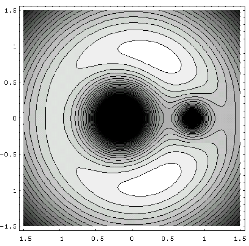
\(\text{FIGURE XVI.8}\)

Figure \(\text{XVI.9a}\) shows a three-dimensional drawing of the equivalent potential surface in the plane, also plotted by Mathematica by Mr Fairbairn. Figure \(\text{XVI.9b}\) is a model of the surface, seen from more or less above. This was constructed of wood by Mr David Smith of the University of Victoria, Canada, and photographed by Mr David Balam, also of the University of Victoria. The mass ratio is \(q = 5\).

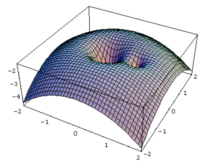
\(\text{FIGURE XVI.9A}\)

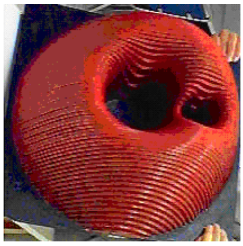
\(\text{FIGURE XVI.9B}\)

We can imagine the path taken by a small particle in the field of the two principal masses by imagining a small ball rolling or sliding on the equivalent potential surface. It might roll into one of the two deep hyperbolic potential wells representing the gravitational attraction of the two masses. Or it might roll down the sides of the big paraboloid – i.e. it might be flung outwards by the effect of centrifugal force. We must remember, however, that the surface represents the equivalent potential referred to a co-rotating frame, and that, whenever the particle moves relative to this frame, it experiences a Coriolis force at right angles to its velocity.

The three collinear lagrangian points are actually saddle points. Along the x-axis (figure XVI.5, they are maxima, but when the potential is plotted parallel to the y-axis, they are minima. However, in this section, we shall be particularly interested in the equilateral points, whose coordinates (verify this) are . \(x_{\text{L}} = \frac{1}{2} \left( \frac{q-1}{q+1} \right) , \ y_{\text{L}} = \pm \frac{\sqrt{3}}{2}\). You may verify from Equations 16.2.4 and 5, (though you may need some patience to do so) that the first derivatives are zero there. Even more patience and determination would be needed to determine from the second derivatives that the equivalent potential is a maximum there – though you may prefer to look at figures \(\text{XVI.8}\) and \(\text{9}\) rather than wade through that algebra. I have done the algebra and I can tell you that the first derivatives at the equilateral points are indeed zero and the second derivatives are as follows.

\[W_{xx} = - \frac{3}{4}, \quad W_{yy} = -\frac{9}{4}, \quad W_{zz} = +1, \quad W_{yz} = W_{zx} = 0, \quad W_{xy} = -\frac{3\sqrt{3}}{4} \left( \frac{q-1}{q+1} \right) . \]

Because \(W_{zz} = +1\), the potential at the equilateral points goes through a minimum as we cross the plane; in the plane, however, \(W\) is a maximum, and it has the value there of

\[-\frac{3q^2 + 5q + 3}{2(q + 1)^2} . \]

In the matter of notation, the equilateral points are often called the fourth and fifth lagrangian points, denoted by \(\text{L}_4\) and \(\text{L}_5\). The question arises, then, which is \(\text{L}_4\) and which is \(\text{L}_5\)? Most authors label the equilateral point that leads the less massive of the two principal masses by \(60^\circ\) \(\text{L}_4\) and the one that trails by \(60^\circ \ \text{L}_5\). This would be unambiguous if we were to restrict our interest, for example, to Trojan asteroids of planets in orbit around the Sun, or Calypso which leads Tethys in orbit around Saturn and Telesto which follows Tethys. There would be ambiguity, however, if the two principal bodies had equal masses, or if the two principal bodies were the members of a close binary pair of stars in which mass transfer led to the more massive star becoming the less massive one. In such special cases, we would have to be careful to make our meaning clear. For the present, however, I shall assume that the two principal bodies have unequal masses, and the equilateral point that precedes the less massive body is \(\text{L}_4\).

In figure \(\text{XVI.10}\) we are looking in the \(xy\)-plane. I have marked a point \(\text{P}\), with coordinates \((x, y, z)\); these are expressed in units of \(a\), the constant separation of the two principal masses. The origin of coordinates is the centre of mass \(\text{C}\), and the coordinates (in units of \(a\)) of the two masses are shown. The angular momentum vector ω is directed along the direction of increasing \(z\).

Now imagine a particle of mass \(m\) at \(\text{P}\). It will be subject to a force given by the negative of the gradient of the potential energy, which is \(m\) times the potential. Thus in the \(x\)-direction, \(ma \ddot{x} = - m \frac{\partial V}{a \partial x}\). In addition to this force, however, whenever it is in motion relative to the co-rotating frame it is subject to a Coriolis force \(2m \textbf{v}×\textbf{ω}\). Thus the \(x\)-component of the Equation of motion is \(ma \ddot{x} = -m \frac{\partial V}{a \partial x} + 2mω a \dot{y}\). Dividing through by \(ma\) we find for the Equation of motion in the \(x\)-direction

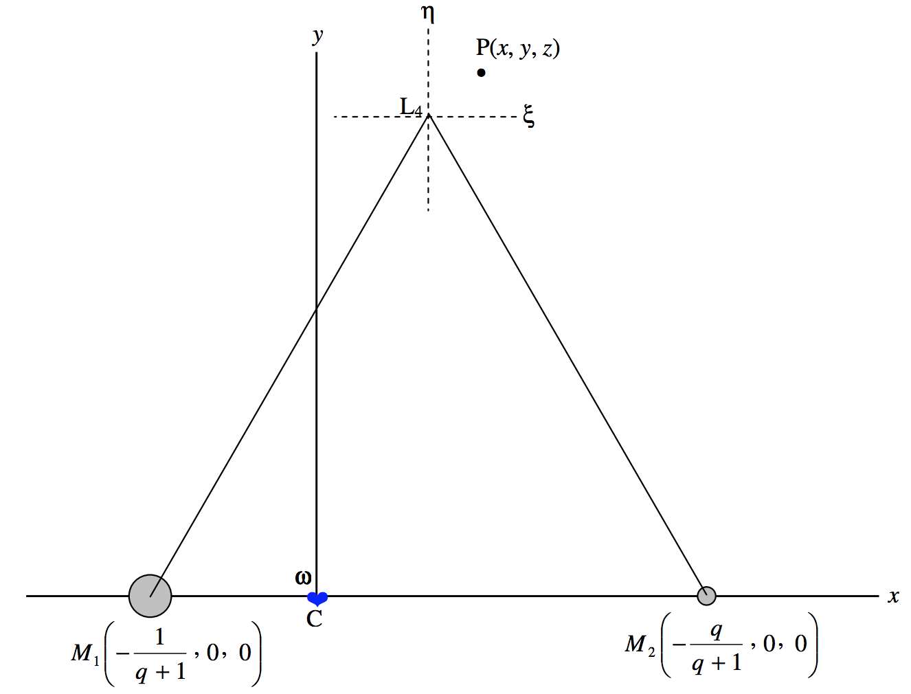
\(\text{FIGURE XVI.10}\)

\[\ddot{x} = -\frac{1}{a^2} \frac{\partial V}{\partial x} + 2ω \dot{y} . \label{16.2.13} \tag{16.2.13}\]

Similarly in the other two directions, we have

\[\ddot{y} = -\frac{1}{a^2} \frac{\partial V}{\partial y} - 2ω \dot{x} \label{16.2.14} \tag{16.2.14}\]

and \[\ddot{z} = -\frac{1}{a^2} \frac{\partial V}{\partial z}. \label{16.2.15} \tag{16.2.15}\]

These, then, are the differential Equations that will track the motion of a particle moving in the vicinity of the two principal orbiting masses. For large excursions, they are best solved numerically. However, solutions close to the equilateral points lend themselves to a simple analytical solution, which we shall attempt here. Let us start, then, by referring positions to coordinates with origin at an equatorial lagrangian point. The coordinates of the point \(\text{P}\) with respect to the lagrangian point are \((ξ, η, ζ )\), where \(ξ = x - x_L , \ η = y - y_L, ζ = z\). Note also that \(\dot{ξ} = \dot{x} \ \ddot{ξ} =\ddot{x}\), etc. We are going to need the derivatives of the potential near to the lagrangian points, and, by Taylor’s theorem (or just common sense!) these are given by

\[V_x = (V_x )_\text{L} + ξ (V_{xx} )_\text{L} + η (V_{yx})_\text{L} + ζ (V_{zx} )_\text{L} , \label{16.2.16} \tag{16.2.16}\]

\[V_y = (V_y )_\text{L} + ξ (V_{xy} )_\text{L} + η (V_{yy})_\text{L} + ζ (V_{zy} )_\text{L} , \label{16.2.17} \tag{16.2.17}\]

\[V_z = (V_z )_\text{L} + ξ (V_{xz} )_\text{L} + η (V_{yz})_\text{L} + ζ (V_{zz} )_\text{L} , \label{16.2.18} \tag{16.2.18}\]

We have already worked out the derivatives at the lagrangian points (the first derivatives are zero), so now we can put these expressions into Equations 16.2.13,14 and 15, to obtain

\[\ddot{ξ} - 2ω \dot{η} = ω^2 \left( \frac{3}{4} ξ + \frac{3 \sqrt{3} (q-1)}{4(q+1)} η \right) , \label{16.2.19} \tag{16.2.19}\]

\[\ddot{η} + 2ω\dot{ξ} = ω^2 \left( \frac{3\sqrt{3}(q-1)}{4(q+1)}ξ + \frac{9}{4} η \right) \label{16.2.20} \tag{16.2.20}\]

and \[\ddot{ζ} = - ω^2 ζ . \label{16.2.21} \tag{16.2.21}\]

The last of these Equations tells us that displacements in the \(z\)-direction are periodic with period equal to the period of the two principal orbiting bodies. The motion is bounded and stable perpendicular to the plane. An orbit inclined to the plane of the orbits containing \(M_1\) and \(M_2\) is stable.

For ξ and η, let us seek periodic solutions of the form

\[\ddot{ξ} = n^2 ξ \text{ and } \ddot{η} = n^2 η \label{16.2.22a,b} \tag{16.2.22a,b}\]

so that

\[\dot{ξ} = in ξ \text{ and } \dot{η} = in η \label{16.2.23a,b} \tag{16.2.23a,b}\]

where \(n\) is real and therefore \(n^2\) is positive.

Substitution of these in Equations 16.2.19-21 gives

\[(n^2 + \frac{3}{4} ω^2) ξ + \left( wωni + \frac{3\sqrt{3}}{4} \left( \frac{q-1}{q+1} \right) ω^2 \right) η = 0 \label{16.2.24} \tag{16.2.24}\]

and \[\left( 2ω ni - \frac{3\sqrt{3}}{4} \left( \frac{q-1}{q+1} \right) ω^2 \right)ξ - (n^2 + \frac{9}{4} ω^2 ) η = 0. \label{16.2.25} \tag{16.2.25}\]

A trivial solution is \(ξ = η = 0\); that is, the particle is stationary at the lagrangian point. While this is indeed a possible solution, it is unstable, since the potential is a maximum there. Nontrivial solutions are found by setting the determinant of the coefficients equal to zero. Thus

\[n^4 - ω^2 n^2 + \frac{27qω^4}{4(q+1)^2} = 0 . \label{16.2.26} \tag{16.2.26}\]

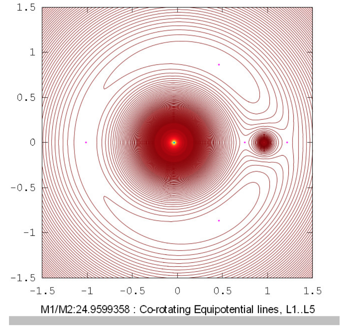
This is a quadratic Equation in \(n^2\), and for real \(n^2\) we must have \(b^2 > 4ac\), or \(1 > \frac{27q}{(q+1)^2}\), or \(q^2 - 25q + 1 >0\). That is, \(q > 24.959 \ 935 \ 8\) or \(q < 1/24.959 \ 935 \ 8 = 0.040 \ 064 \ 206\). We also require \(n^2\) to be not only real but positive. The solutions of Equation \(16.2.26\) are

\[2n^2 = ω^2 \left( 1 \pm \sqrt{1 - 27q/(1+q)^2} \right) . \label{16.2.27} \tag{16.2.27}\]

For any mass ratio \(q\) that is less than \(0.040 \ 064 \ 206\) or greater than \(24.959 \ 935 \ 8\) both of these solutions are positive. Thus stable elliptical orbits (in the co-rotating frame) around the equilateral lagrangian points are possible if the mass ratio of the two principal masses is greater than about 25, but not otherwise.

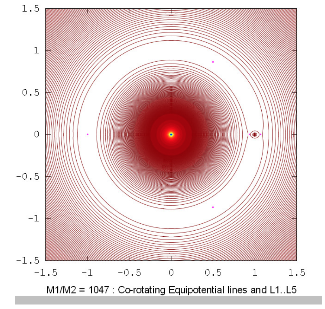
If we consider the Sun-Jupiter system, for which \(q = 1047.35\), we have that

\(n = 0.996 757ω \text{ or } n = 0.080 464 5ω.\)

The period of the motion around the lagrangian point is then

\(P = 1.0033P_{\text{J}} \text{ or } P = 12.428P_\text{J}\)

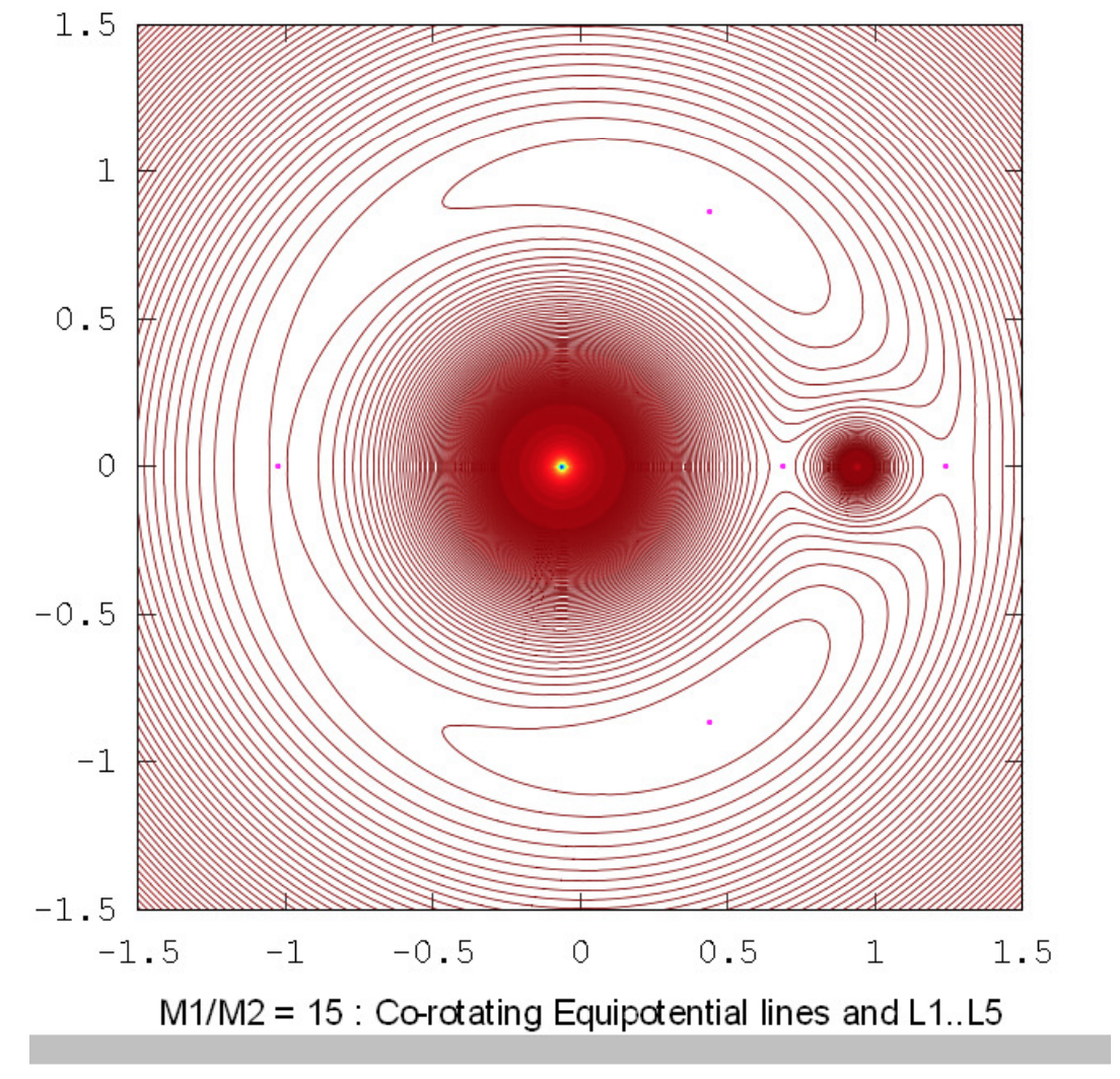
This description of the motion applies to asteroids moving closely around the equilateral lagrangian points, and the approximation made in the analysis appeared in the Taylor expansion for the potential given by Equations 16.2.16-18. For more distant excursions one might try analytical solutions by expanding the Taylor series to higher-order terms (and of course working out the higher-order derivatives) or it might be easier to integrate Equations 16.2.19 and 20 numerically. Many people have had an enormous amount of fun with this. The orbits do not follow the equipotential contours exactly, of course, but in general shape they are not very different in appearance from the contours. Thus, for larger excursions from the lagrangian points the orbits become stretched out with a narrow tail curving towards \(\text{L}_1\); such orbits bear a fanciful resemblance to a tadpole shape and are often referred to as tadpole orbits. For yet further excursions, an asteroid may start near \(\text{L}_4\) and roll downhill, veering around the back of the more massive body, through the \(\text{L}_1\) point and then upwards towards \(\text{L}_5\); then it slips back again, goes again through \(\text{L}_1\) and then up to \(\text{L}_4\) again – and so on. This is a so-called horseshoe orbit.

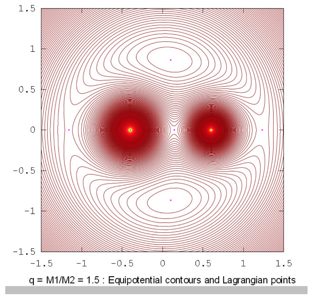
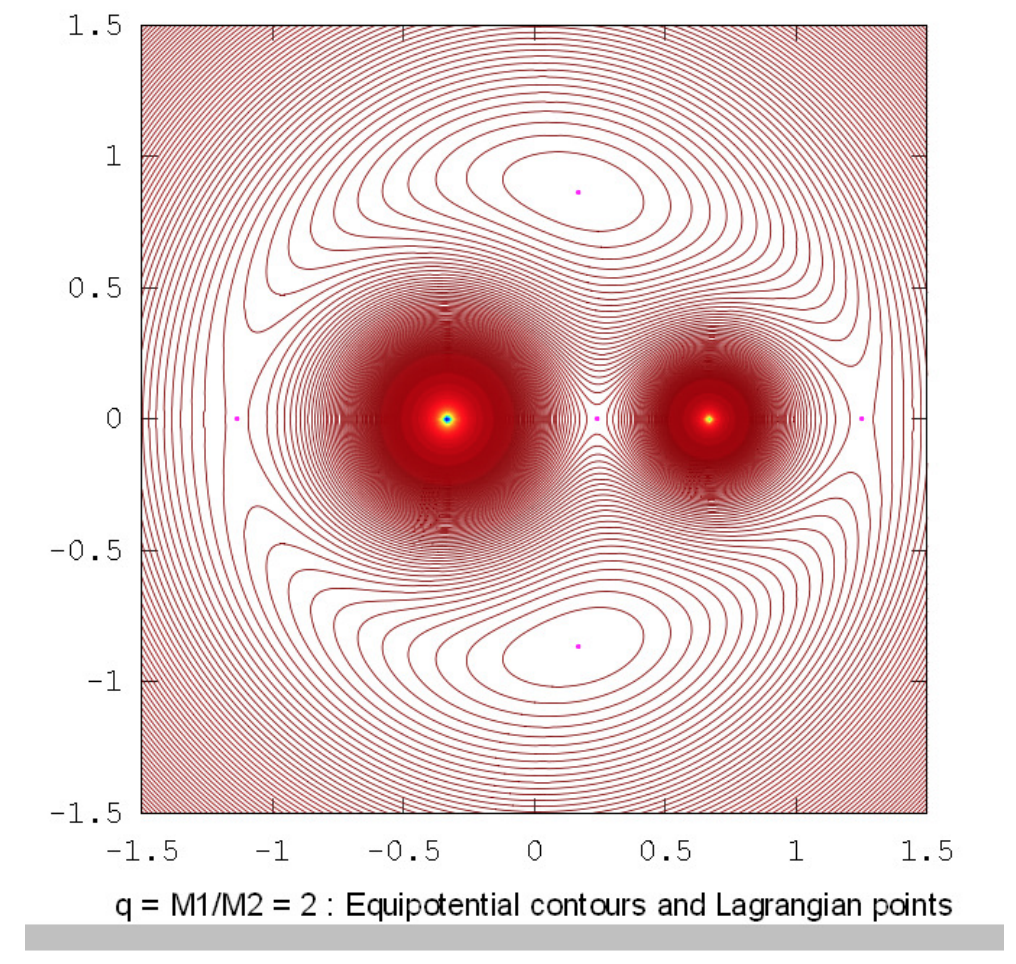
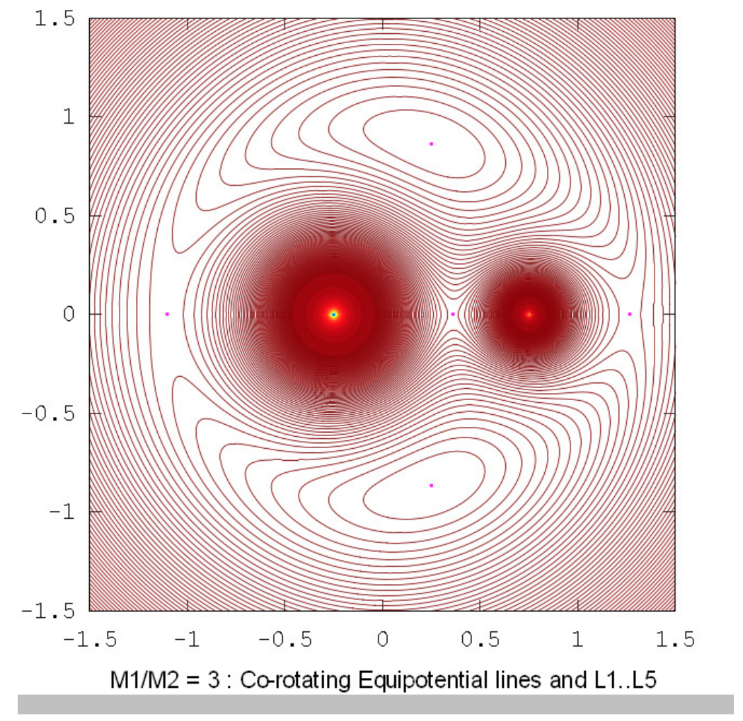
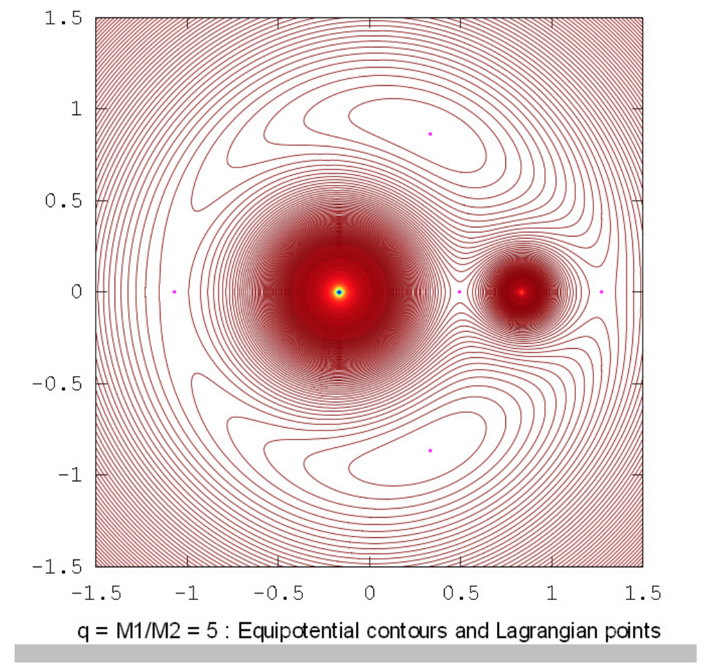
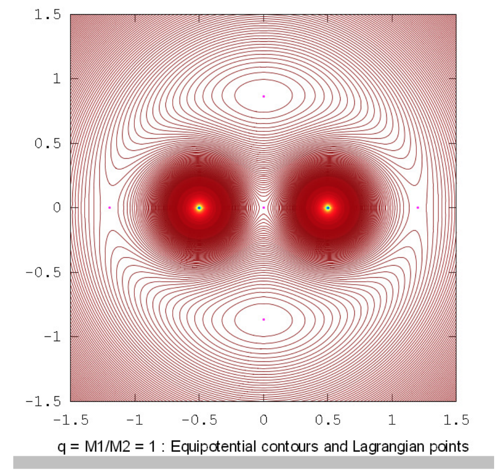
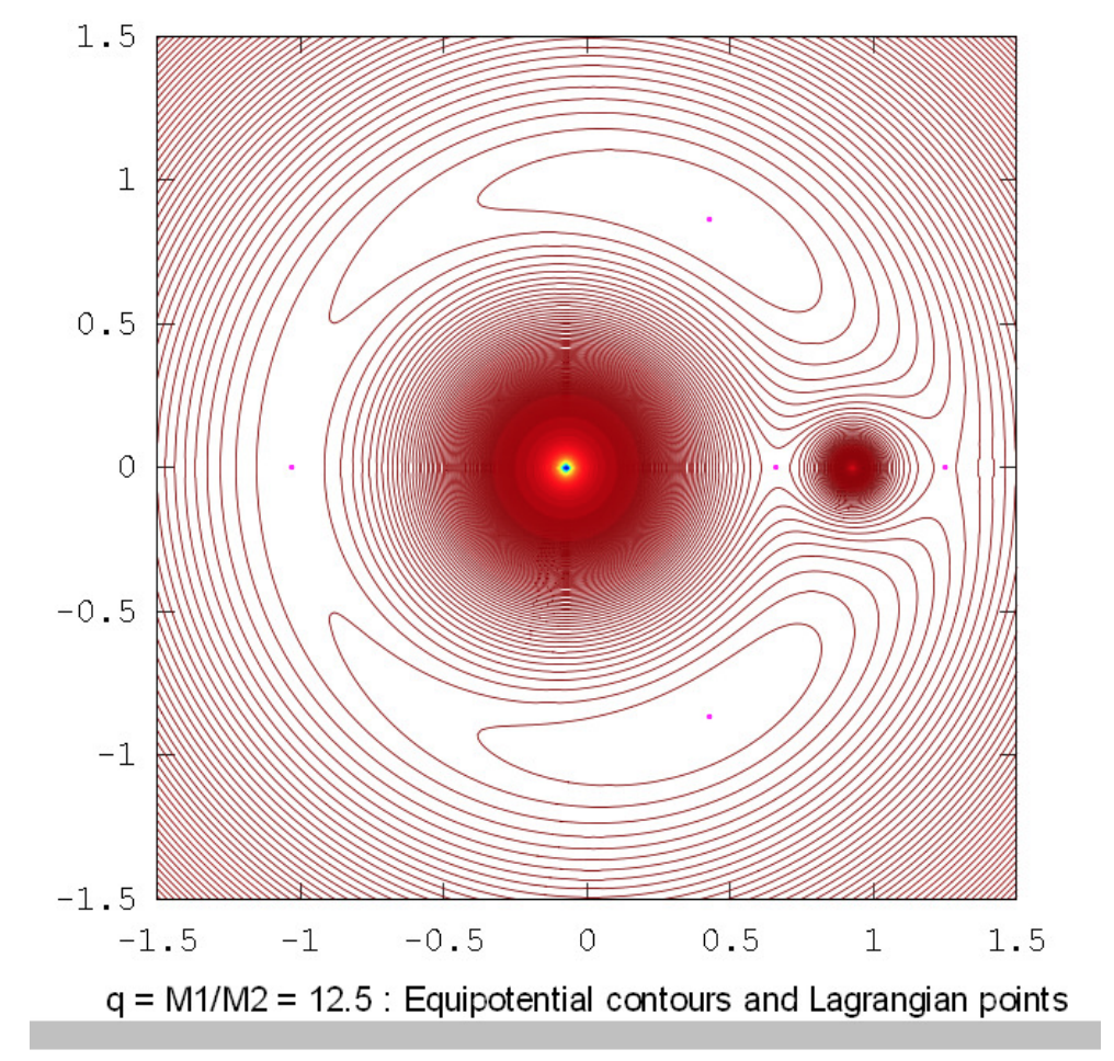
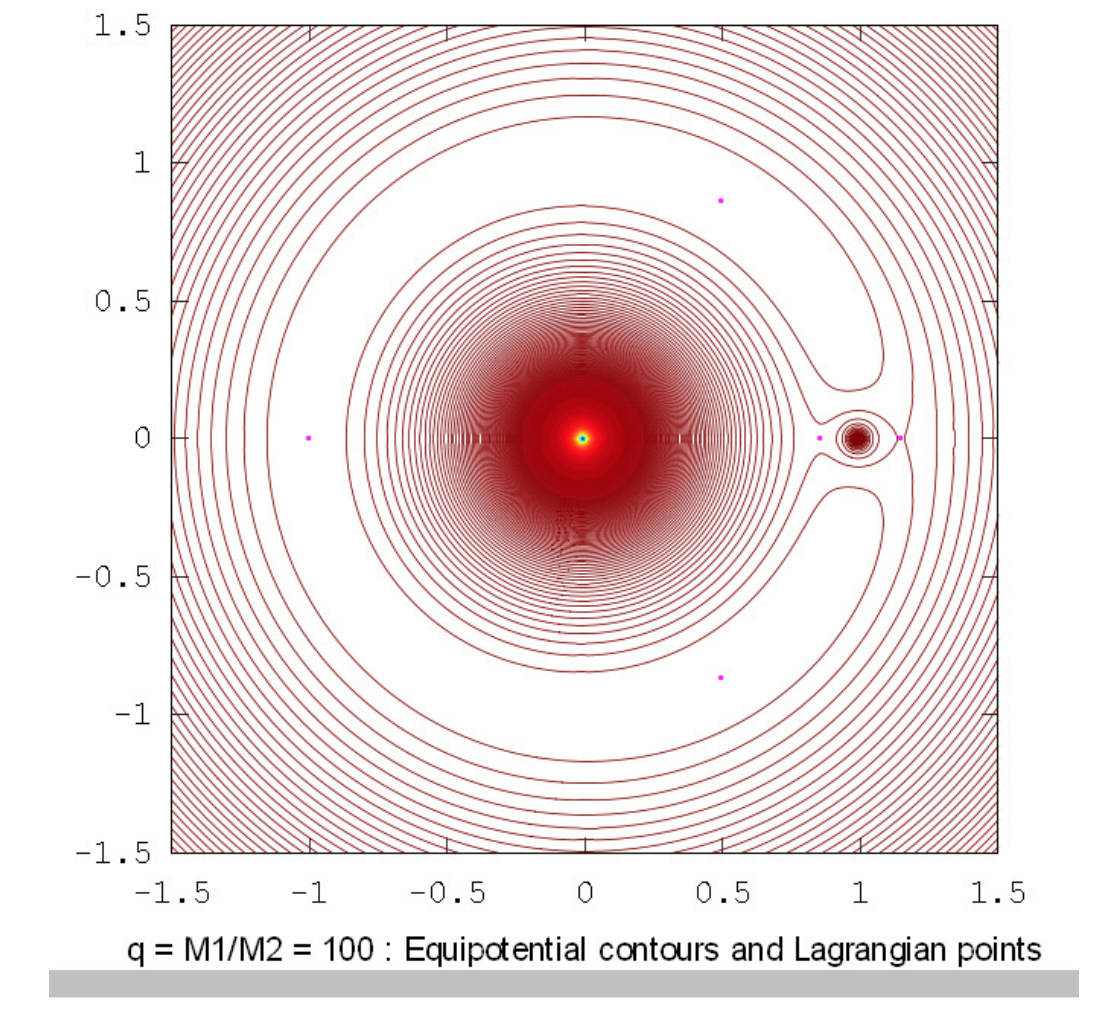
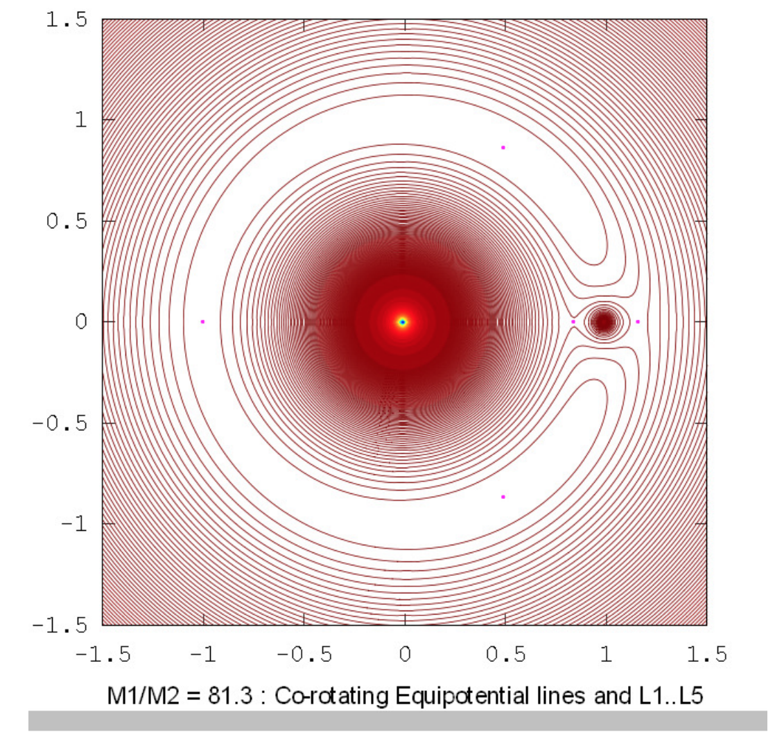
The drawings below show the equipotential contours for a number of mass ratios. These drawings were prepared using Octave by Dr Mandayam Anandaram of Bangalore University, and are dedicated by him to the late Max Fairbairn of Sydney, Australia, who prepared figures \(\text{XVI.8}\) and \(\text{XVI.9a}\) for me shortly before his untimely death. Anand and Max were my first graduate students at the University of Victoria, Canada, many years ago. These drawings show the gradual evolution from tadpole-shaped contours to horseshoe-shaped contours. The mass-ratio \(q = 24.959 \ 935 \ 8\) is the critical ratio below which stable orbits around the equilateral points \(\text{L}_4\) and \(\text{L}_5\) are not possible. The massratios \(q = 81.3\) and \(1047\) are the ratios for the Earth-Moon and Sun-Jupiter systems respectively. The reader will notice that, in places where the contours are closely-spaced, in particular close to the deep potential well of the larger mass, Moiré fringes appear. These fringes appear where the contour separation is comparable to the pixel size, and the reader will recognize them as Moiré fringes and, we think, will not be misled by them.

Dr Anandaram has also prepared a number of fascinating drawings in which sample orbits are superimposed, in a second colour, on the equipotential contours. These include tadpole orbits in the vicinity of the equilateral points; “triangular” orbits of the Hilda asteroids, which are in 2 : 3 resonance with Jupiter; the almost “square” orbit of Thule, which is in 3 : 4 resonance with Jupiter; and half of a complete 9940 year libration period of Pluto, which is in 3 : 2 resonance with Neptune. It is proposed to publish these in a separate paper dedicated to Max, the reference to which will in due course be given in these notes.