1.12: Fitting a Least Squares Straight Line to a Set of Observational Points

Very often we have a set of observational points \((x_i , y_i), \ i = 1\) to \(N\), that seem to fall roughly but not quite on a straight line, and we wish to draw the “best” straight line that passes as close as possible to all the points. Even the smallest of scientific hand calculators these days have programs for doing this – but it is well to understand precisely what it is that is being calculated.

Very often the values of \(x_i\) are known “exactly” (or at least to a high degree of precision) but there are appreciable errors in the values of \(y_i\). In figure \(\text{I.6B}\) I show a set of points and a plausible straight line that passes close to the points.

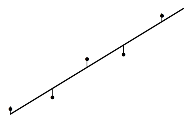
\(\text{FIGURE I.6B}\)

Also drawn are the vertical distances from each point from the straight line; these distances are the residuals of each point.

It is usual to choose as the “best” straight line that line such that the sum of the squares of these residuals is least. You may well ask whether it might make at least equal sense to choose as the “best” straight line that line such that the sum of the absolute values of the residuals is least. That certainly does make good sense, and in some circumstances it may even be the appropriate line to choose. However, the “least squares” straight line is rather easier to calculate and is readily amenable to statistical analysis. Note also that using the vertical distances between the points and the straight line is appropriate only if the values of \(x_i\) are known to much higher precision than the values of \(y_i\). In practice, this is often the case – but it is not always so, in which case this would not be the appropriate “best” line to choose.

The line so described – i.e. the line such that the sum of the squares of the vertical residuals is least is often called loosely the “least squares straight line”. Technically, it is the least squares linear regression of \(y\) upon \(x\). It might be under some circumstances that it is the values of \(y_i\) that are known with great precision, whereas there may be appreciable errors in the \(x_i\). In that case we want to minimize the sum of the squares of the horizontal residuals, and we then calculate the least squares linear regression of \(x\) upon \(y\). Yet again, we may have a situation in which the errors in \(x\) and \(y\) are comparable (not necessarily exactly equal). In that case we may want to minimize the sum of the squares of the perpendicular residuals of the points from the line. But then there is a difficulty of drawing the \(x\)- and \(y\)-axes to equal scales, which would be problematic if, for example, \(x\) were a time and \(y\) a distance.

To start with, however, we shall assume that the errors in \(x\) are negligible and we want to calculate the least squares regression of \(y\) upon \(x\). We shall also make the assumption that all points have equal weight. If they do not, this is easily dealt with in an obvious manner; thus, if a point has twice the weight of other points, just count that point twice.

So, let us suppose that we have \(N\) points, \((x_i , y_i)\), \(i = 1\) to \(N\), and we wish to fit a straight line that goes as close as possible to all the points. Let the line be \(y=a_1 x + a_0\). The residual \(R_i\) of the \(i\)th point is

\[R_i = y_i - (a_1 x_i + a_0) . \label{1.12.1} \tag{1.12.1}\]

We have \(N\) simultaneous linear Equations of this sort for the two unknowns \(a_1\) and \(a_0\), and, for the least squares regression of \(y\) upon \(x,\) we have to find the values of \(a_1\) and \(a_0\) such that the sum of the squares of the residuals is least. We already know how to do this from Section 1.8, so the problem is solved. (Just make sure that you understand that, in Section 1.8 we were using \(x\) for the unknowns and \(a\) for the coefficients; here we are doing the opposite!)

Now for an Exercise. Suppose our points are as follows:

\begin{array}{c c}
x & y \\
\\
1 & 1.00 \\
2 & 2.50 \\
3 & 2.75 \\
4 & 3.00 \\
5 & 3.50 \\
\end{array}

i.) Draw these points on a sheet of graph paper and, using your eye and a ruler, draw what you think is the best straight line passing close to these points.

ii.) Write a computer program for calculating the least squares regression of \(y\) upon \(x\). You’ve got to do this sooner or later, so you might as well do it now. In fact you should already (after you read Section 1.8) have written a program for solving \(N\) Equations in \(n\) unknowns, so you just incorporate that program into this.

iii.) Now calculate the least squares regression of \(y\) upon \(x\). I make it \(y = 0.55x + 0.90\). Draw this on your graph paper and see how close your eye-and-ruler estimate was!

iv.) How are you going to calculate the least squares regression of \(x\) upon \(y\)? Easy! Just use the same program, but read the \(x\)-values for \(y\) and the \(y\)-values for \(x\)! No need to write a second program! I make it \(y = 0.645x + 0.613\). Draw that on your graph paper and see how it compares with the regression of \(y\) upon \(x\).

The two regression lines intersect at the centroid of the points, which in this case is at (3.00, 2.55). If the errors in \(x\) and \(y\) are comparable, a reasonable best line might be one that passes through the centroid, and whose slope is the mean (arithmetic? geometric?) of the regressions of \(y\) upon \(x\) and \(x\) upon \(y\). However, in Section 1.12 I shall give a reference to where this question is treated more thoroughly.

If the regressions of \(y\) upon \(x\) and \(x\) upon \(y\) are respectively \(y = a_1 x + a_0\) and \(y = b_1 x + b_0\), the quantity \(\sqrt{a_1/b_1}\) is called the correlation coefficient r between the variates x and y. If the points are exactly on a straight line, the correlation coefficient is 1. The correlation coefficient is often used to show how well, or how badly, two variates are correlated, and it is often averred that they are highly correlated if \(r\) is close to 1 and only weakly correlated if \(r\) is close to zero. I am not intending to get bogged down in formal statistics in this chapter, but a word of warning here is in order. If you have just two points, they are necessarily on a straight line, and the correlation coefficient is necessarily 1 – but there is no evidence whatever that the variates are in any way correlated. The correlation coefficient by itself does not tell how closely correlated two variates are. The significance of the correlation coefficient depends on the number of points, and the significance is something that can be calculated numerically by precise statistical tests.