6.2: Solving the 1D Infinite Square Well

Imagine a (non-relativistic) particle trapped in a one-dimensional well of length \(L\). Inside the well there is no potential energy, and the particle is trapped inside the well by “walls” of infinite potential energy.

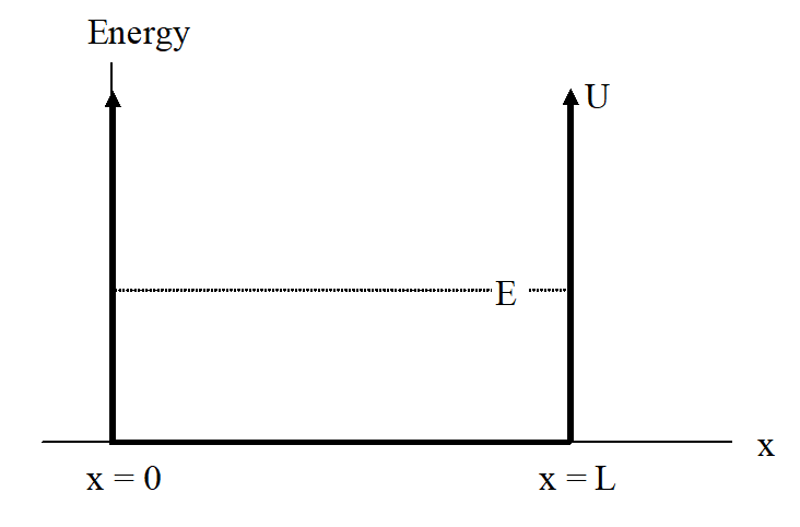
Figure \(\PageIndex{1}\)

Since this potential is a piece-wise function, Schrödinger’s equation must be solved in the three regions separately. In the region \(x >L\) (and \(x < 0\)), the equation is:

\[ - \dfrac{\hbar^2}{2m} \dfrac{d}{dx^2} \psi(x) + U(x)\psi x = E \psi(x) \label{eq1}\]

\[-\frac{h^2}{2 m} \frac{d^2}{d x^2} \psi(x)+(\infty) \psi(x)=E \psi(x)\]

\[(\infty) \psi(x)=E \psi(x)\]

This has solutions of \(E = ∞\), which is impossible (no particle can have infinite energy) or \(\psi = 0\). Since \(\psi=0\), the particle can never be found outside of the well.

In the region \(0 < x < L\), the equation is:

\[\begin{array}{l}-\frac{h^2}{2 m} \frac{d^2}{d x^2} \psi(x)+U(x) \psi(x)=E \psi(x) \\ -\frac{h^2}{2 m} \frac{d^2}{d x^2} \psi(x)+(0) \psi(x)=E \psi(x) \\ -\frac{h^2}{2 m} \frac{d^2}{d x^2} \psi(x)=E \psi(x) \\ \frac{d^2}{d x^2} \psi(x)=-\frac{2 m E}{h^2} \psi(x)\end{array}\]

The general solution to this equation is

\(\psi(x)=A \sin (k x)+B \cos (k x)\) with \(\quad k=\sqrt{\frac{2 m E}{h^2}}\)

The solutions in the different regions of space must be continuous across the boundaries at \(x = 0\) and \(x = L\) (the derivatives of the solutions must also be continuous if the potential energy is continuous at these points).

At \(x = 0\), equate the two solutions:

\[\begin{array}{l}\psi\left(x=0^{-}\right)=\psi\left(x=0^{+}\right) \\ 0=A \sin (k 0)+B \cos (k 0) \\ 0=\mathrm{B}\end{array}\]

therefore, the cosine portion of the solution has amplitude zero.

At \(x = L\), equate the two solutions:

\[\begin{array}{l}\psi\left(x=L^{-}\right)=\psi\left(x=L^{+}\right) \\ A \sin (k L)=0 \\ k L=n \pi \\ k=\frac{n \pi}{L}\end{array}\]

This leads to allowed wavefunctions:

\[\psi(x)=A \sin \left(\frac{n \pi x}{L}\right)\]

and allowed energies:

\[\begin{array}{l}k=\sqrt{\frac{2 m E}{h^2}} \\ \left(\frac{n \pi}{L}\right)^2=\frac{2 m E}{h^2} \\ \left(\frac{n \pi}{L}\right)^2=\left(\frac{2 \pi}{h}\right)^2 2 m E \\ E=\frac{n^2 h^2}{8 m L^2} \\ E=n^2 \frac{(h c)^2}{8 m c^2 L^2}\end{array}\]

These solutions are represented below. On the left is the standard textbook representation, where the wavefunction is superimposed on the graph of energy. Remember, however, that what is “waving” above and below the energy level isn’t a measure of energy (i.e., the energy is a constant value at each level), but rather related to the probability of finding the particle at each location in space. The representation on the right tries to represent the regions where it is more likely to find the particle (the darker regions) and the regions where it is less likely to find the particle.

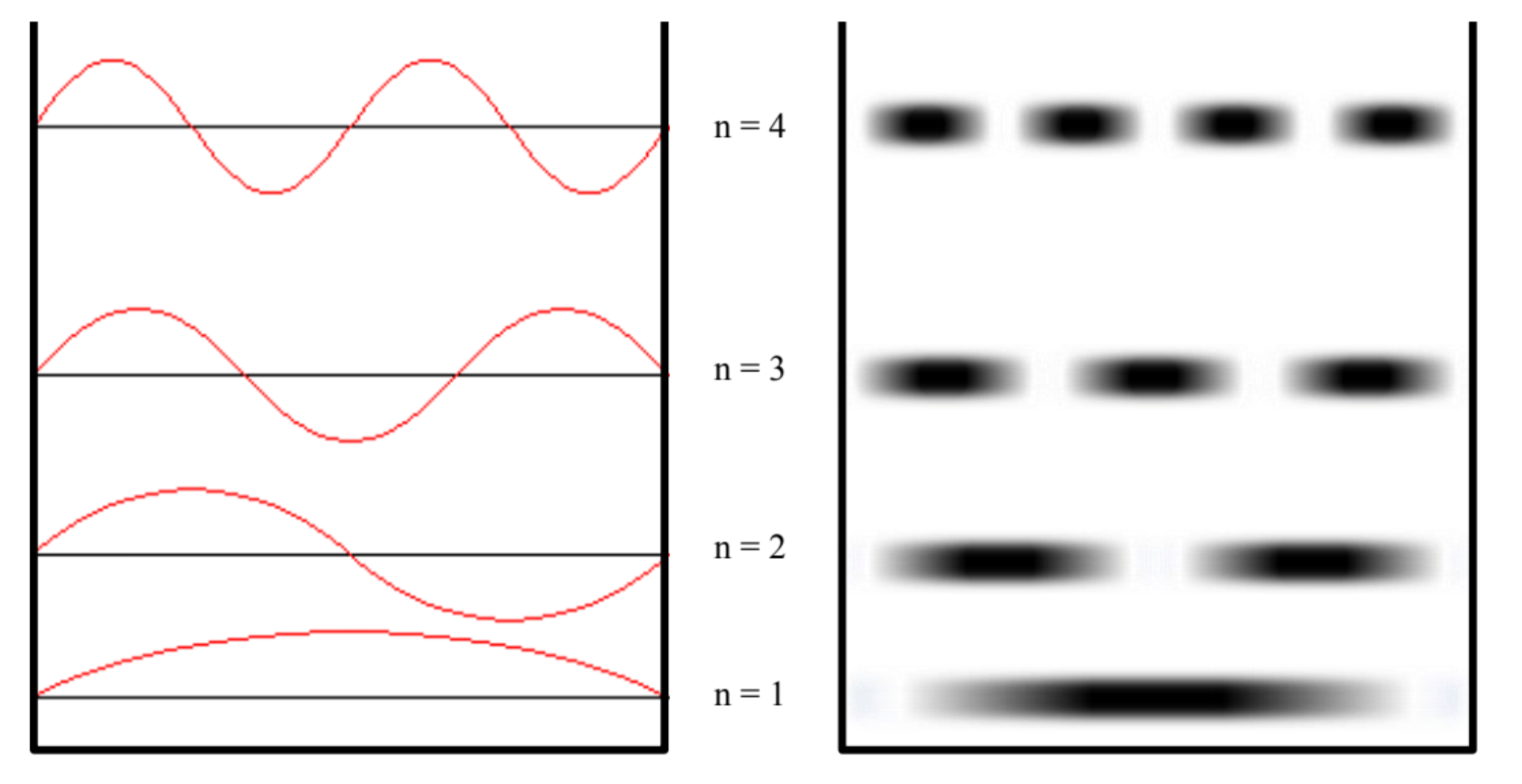
Figure \(\PageIndex{1}\): To the left the wavefunction, to the right a representation of the probability of finding the particle at a specific position for the various quantum states.

 

Additionally, since the probability of finding the particle somewhere in the well is equal to 1, and the probability of finding the particle is equal to the wavefunction squared,

using an integral table yields the result

This result has a number of extremely important features.

• The particle can only have certain, discrete values for energy. In classical physics, a particle trapped in a region of space can have any, continuous value for energy. The restriction of a bound particle to specific, quantized values of allowed energy is a hallmark of quantum mechanics.
• The particle cannot be at rest. Notice that the lowest possible energy for the particle is in the \(n = 1\) state, which has non-zero energy. This is termed the zero-point energy, and can be understood as a consequence of the Heisenberg uncertainty principle. This is in complete contrast to classical physics.
• The particle has regions of high and low probability of being found in the well. The probability of finding the particle is equal to the square of the wavefunction, which is not a constant value. Unlike classical physics, where the particle is equally likely to be anywhere in the well, in quantum mechanics there exist positions where the particle will never be found, and regions where the probability of finding the particle is greatly enhanced. for example, in the \(n = 2\) state, the particle will never be found in the center of the well, while it is very likely to find the particle at the positions \(x = L/4\) and \(x = 3L/4\).

The 1D Infinite Well

An electron is trapped in a one-dimensional infinite potential well of length \(4.0 \times 10^{-10}\, m\). Find the three longest wavelength photons emitted by the electron as it changes energy levels in the well.

The allowed energy states of a particle of mass m trapped in an infinite potential well of length L are
\[ E = n^2\frac{(hc)^2}{8mc^2L^2} \]

Therefore, the electron has allowed energy levels given by
\[ \begin{array}{rcl} E & = & n^2\frac{(hc)^2}{8mc^2L^2} \\E & = & n^2\frac{(1240)^2}{8(511000 \text{eV})(0.4 \text{nm})^2} \\ E & = & n^2 (2.35 \text{eV}) \end{array}\]

As the electron changes energy levels, the energy released by the electron is in the form of a photon.
\[\begin{array}{rl} E_{photon} &= E_{initial \ electron} - E_{final \ electron} \\ E_{photon} &= (n_i^2 - n_f^2) 2.35 \text{eV} \end{array}\]

Thus, the emitted wavelengths are
\[\begin{array}{rcl} \lambda &=& \frac{hc}{E_{photon}} \\ \lambda &=& \frac{1240 \text{eV nm}}{(n_i^2 - n_f^2)2.35 \text{eV nm}} \\ \lambda &=& \frac{528 \text{ nm}}{(n_i^2 - n_f^2)} \end{array}\]

The longest wavelength photons involve the smallest value of \(n_i^2 - n_f^2\). These are:
\[ \begin{array}{ccc} n_i & n_f & \lambda \\ \hline \\ 2 & 1 & 176 \text{nm} \\ 3 & 2 & 106\text{ nm} \\ 4 & 3 & 75.6 \text{ nm} \end{array}\]