
4.5: Euler's Equations of Motion
- Page ID
- 6950

In our first introduction to classical mechanics, we learn that when an external torque acts on a body its angular momentum changes (and if no external torques act on a body its angular momentum does not change.) We learn that the rate of change of angular momentum is equal to the applied torque. In the first simple examples that we typically meet, a symmetrical body is rotating about an axis of symmetry, and the torque is also applied about this same axis. The angular momentum is just \( I\omega\), and so the statement that torque equals rate of change of angular momentum is merely \( \tau = I \dot{\omega}\) and that’s all there is to it.
Later, we learn that \( \bf{L}\) = \( I \boldsymbol\omega\), where \( \bf{l}\) is a tensor, and \( \bf{L}\) and \( \boldsymbol\omega\) are not parallel. There are three principal moments of inertia, and \( \bf{L}\), \( \boldsymbol\omega\) and the applied torque \( \boldsymbol\tau \) each have three components, and the statement “torque equals rate of change of angular momentum” somehow becomes much less easy.
Euler’s Equations sort this out, and give us a relation between the components of the \( \boldsymbol\tau \), \( \bf{l}\) and \( \boldsymbol\omega\).
For Figure IV.5, I have just reproduced, with some small modifications, Figure III.19 from my notes on this Web site on Celestial Mechanics, where I defined Eulerian angles. Again it is suggested that those who are unfamiliar with Eulerian angles consult Chapter III of Celestial Mechanics.
In Figure IV.5, \( Oxyz\) are space-fixed axes, and \( Ox_{0}y_{0}z_{0}\) are the body-fixed principal axes. The axis \( Oy_{0}\) is behind the plane of your screen; you will have to look inside your monitor to find it.

I suppose an external torque \( \boldsymbol\tau \) acts on the body, and I have drawn the components \( \tau_{1} \) and \( \tau_{3} \). Now let’s suppose that the body rotates in such a manner that the Eulerian angle \( \psi \) were to increase by \( \delta\psi\) . I think it will be readily agreed that the work done on the body is \( \tau_{3}\delta\psi\). This means, following our definition of generalized force in Section 4.4, that \( \tau_{3} \) is the generalized force associated with the generalized coordinate \( \psi\). Having established that, we can now apply the Lagrangian Equation 4.4.1:
\[ \ \frac{\text{d}}{\text{d}t} (\frac{\partial T}{\partial \dot{\psi}})-\frac{\partial T}{\partial \psi} = \tau_{3} \tag{4.5.1}\label{eq:4.5.1} \]
Here the kinetic energy is the expression that we have already established in Equation 4.3.6. In spite of the somewhat fearsome aspect of Equation 4.3.6, it is quite easy to apply Equation \( \ref{eq:4.5.1}\) to it. Thus
\[ \ \frac{\partial T}{\partial \dot{\psi}}= I_{3}(\dot{\phi}cos\theta + \psi) = I_{3}\omega \tag{4.5.2}\label{eq:4.5.2} \]
where I have made use of Equation 4.2.3.
Therefore
\[ \ \frac{\text{d}}{\text{d}t}(\frac{\partial T}{\partial \dot{\psi}}) = I_{3}\dot{\omega_{3}} \tag{4.5.3}\label{eq:4.5.3} \]
And, if we make use of Equations 4.2.1,2,3, it is easy to obtain
\[ \ \frac{\partial T}{\partial \psi}) = I_{1}\omega_{1}\omega_{2}- I_{2}\omega_{2}\omega_{2} = \omega_{1}\omega_{2}(I_{1}-I_{2}) \tag{4.5.4}\label{eq:4.5.4} \]
Thus Equation \( \ref{eq:4.5.1}\) becomes:
\[ \ I_{3}\dot{\omega_{3}} - (I_{1} -I_{2})\omega_{1}\omega_{1} = \tau_{3} \tag{4.5.5}\label{eq:4.5.5} \]
This is one of the Eulerian Equations of motion.
Now, although we saw that \( \tau_{3}\) is the generalized force associated with the coordinate y, it will we equally clear that \( \tau_{1}\) is not the generalized force associated with q, nor is \( \tau_{2}\) the generalized force associated with \( \phi \). However, we do not have to think about what the generalized forces associated with these two coordinates are; it is much easier than that. To obtain the remaining two Eulerian Equations, all that is necessary is to carry out a cyclic permutation of the subscripts in Equation \( \ref{eq:4.5.5}\). Thus the three Eulerian Equation are:
\[ \ I_{1}\dot{\omega_{1}} - (I_{2}-I_{2})\omega_{2}\omega_{3} = \tau_{1} , \tag{4.5.6}\label{eq:4.5.6} \]
\[ \ I_{2}\dot{\omega_{2}} - (I_{3}-I_{1})\omega_{3}\omega_{1} = \tau_{2} , \tag{4.5.7}\label{eq:4.5.7} \]
\[ \ I_{3}\dot{\omega_{3}} - (I_{1}-I_{2})\omega_{1}\omega_{2} = \tau_{3} . \tag{4.5.8}\label{eq:4.5.8} \]
These take the place of \( \tau = I \dot{\omega}\) which we are more familiar with in elementary problems in which a body is rotating about a principal axis and a torque is applied around that principal axis.
If there are no external torques acting on the body, then we have Euler’s Equations of free rotation of a rigid body:
\[ \ I_{1}\dot{\omega_{1}} = (I_{2}-I_{3})\omega_{2}\omega_{3} , \tag{4.5.9}\label{eq:4.5.9} \]
\[ \ I_{1}\dot{\omega_{2}} = (I_{3}-I_{1})\omega_{3}\omega_{1} , \tag{4.5.10}\label{eq:4.5.10} \]
\[ \ I_{3}\dot{\omega_{3}} = (I_{1}-I_{2})\omega_{1}\omega_{2} . \tag{4.5.11}\label{eq:4.5.11} \]
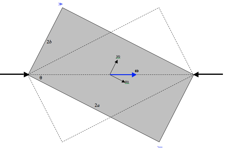
In the above drawing, a rectangular lamina is spinning with constant angular velocity \(\boldsymbol\omega\) between two frictionless bearings. We are going to apply Euler’s Equations of motion to it. We shall find that the bearings are exerting a torque on the rectangle, and the rectangle is exerting a torque on the bearings. The angular momentum of the rectangle is not constant – at least it is not constant in direction. We shall calculate the torque (its magnitude and its direction) and see what is happening to the angular momentum.
We note that the principal (second) moments of inertia are
\( I_{1} = \frac{1}{3}mb^{2} \qquad I_{2} = \frac{1}{3}ma^{2} \qquad I_{3} = \frac{1}{3}m(a^{2} +b^{2})\)
and that the components of angular velocity are
\( \omega_{1} = \omega \cos \theta \qquad \omega_{2} = \omega \sin \theta \qquad \omega_{3} = 0.\)
Also, \(\dot{\boldsymbol\omega}\) and all of its components are zero. We immediately obtain, from Euler’s Equations, that \( \tau_{1}\) and \( \tau_{2}\) are zero, and that the torque exerted on the rectangle by the bearings is
\( \tau_{3} = (I_{2}-I_{1})\omega_{1}\omega_{2} = \frac{1}{3}m(a^{2}-b^{2})\omega^{2}sin \theta \cos \theta\)
And since
\( \sin \theta = \frac{b}{\sqrt{a^{2} +b^{2}}} \quad and \quad \cos \theta = \frac{b}{\sqrt{a^{2} +b^{2}}},\)
we obtain
\( \tau_{3} = \frac{m(a^{2} - b^{2})ab}{3(a^{2} + b^{2})}\omega^{2}\)
Thus \( \boldsymbol\tau \), the torque exerted on the rectangle by the bearings is directed normal to the plane of the rectangle (out of the plane of the paper in the instantaneous snapshot above).
The angular momentum is given by \( { \bf L} = {\bf l} \boldsymbol\omega \). That is to say:
\( \left(\begin{array}{c}L_{1}\\ L_{2}\\L_{3}\end{array}\right) = \frac{1}{3}m\left(\begin{array}{c}b^{2} \quad 0 \quad 0\\ 0 \quad a^{2} \quad 0 \\ 0 \quad 0 \quad a^{2}+b^{2}\end{array}\right)\left(\begin{array}{c}\omega \cos \theta\\ \omega \sin \theta \\ 0\end{array}\right) \)
\( L_{1} = \frac{1}{3}mb^{2}\omega \cos \theta = \frac{1}{3}m\frac{ab^{2}}{\sqrt{a^{2}+b^{2}}}\omega \)
\( L_{2} = \frac{1}{3}mb^{2}\omega \sin \theta = \frac{1}{3}m\frac{ab^{2}}{\sqrt{a^{2}+b^{2}}}\omega \)
\( L_{3} = 0 \)
\( L = \frac{1}{3} mab \omega \)
\( L_{2}/ L_{1} = \frac{a^{2}sin \theta}{b^{2}cos \theta} = \cot \theta = tan(90° - \theta) \)
This tells us that \( \bf L \) is in the plane of the rectangle, and makes an angle 90° - \( \theta \) with the \( x\)-axis, or q with the \( y\)-axis, and it rotates around the vector \( \boldsymbol\tau \). \( \boldsymbol\tau \) is perpendicular to the plane of the rectangle, and of course the change in \( \bf L \) takes place in that direction. The torque does no work, and \( \boldsymbol\omega \) and \( T\) are constant. The reader might find an analogy in the situation of a planet in orbit around the Sun in a circular orbit.. The planet experiences a force that is always perpendicular to its velocity. The force does no work, and the speed and kinetic energy remain constant.
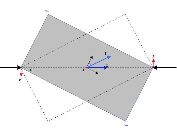
The torque on the plate can be represented as a couple of forces exerted by the bearings on the plate, each of magnitude \( \frac{\tau_{3}}{2\sqrt{a^{2} + b^{2}}}, \) or \( \frac{m(a^{2}-b^{2})}{6(a^{2}-b^{2})^\frac{3}{2}}\omega^{2} \) Forces exerted by the plate on the bearings are, of course, in the opposite direction.
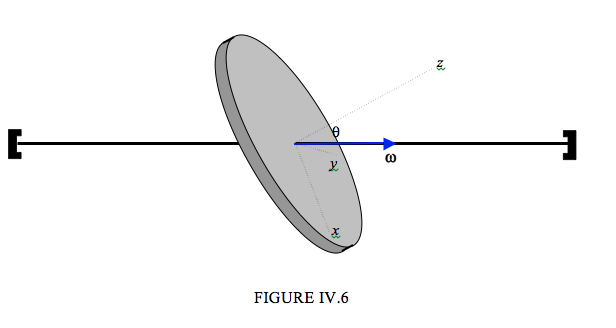
Figure IV.6 shows a disc of mass \( m\), radius \( a\), spinning at a constant angular speed \( \omega\) about at axle that is inclined at an angle \( \theta \) to the normal to the disc. I have drawn three body-fixed principal axes. The \( x\)- and \( y\)- axes are in the plane of the disc\boldsymbol; the direction of the \( x\)-axis is chosen so that the axle (and hence the vector \( \boldsymbol\omega \) ) is in the \( zx\)-plane. The disc is evidently unbalanced and there must be a torque on it to maintain the motion.
Since \( \boldsymbol\omega \) is constant, all components of \( \dot{ \boldsymbol\omega} \) are zero, so that Euler’s Equations are
\( \tau_{1}= (I_{3} - I_{2})\omega_{3}\omega_{2}, \)
\( \tau_{2}= (I_{1} - I_{3})\omega_{1}\omega_{3}, \)
\( \tau_{3}= (I_{2} - I_{1})\omega_{2}\omega_{1}, \)
Now \( \omega_{1} = \omega \sin \theta , \omega_{2} = \omega \cos \theta , I_{1} = \frac{1}{4} ma^{2} , I_{2} = \frac{1}{4} ma^{2}, I_{3} = \frac{1}{1} ma^{2} \)
Therefore \( \tau_{1} = \tau_{3} = 0, and \tau_{2} = - \frac{1}{4}ma^{2}\omega ^{2}sin\theta cos\theta = -\frac{1}{8}ma^{2}\omega^{2}sin2\theta \)
(Check, as always, that this expression is dimensionally correct.) Thus the torque acting on the disc is in the negative \( y\)-direction.
Can you reconcile the fact that there is a torque acting on the disc with the fact that is it moving with constant angular velocity? Yes, most decidedly! What is not constant is the angular momentum \( \bf{L}\), which is moving around the axle in a cone such that \( \dot{\bf L} = -\tau_{2} { \bf j} \), where \( \bf{j}\) is the unit vector along the \( y\)-axis.