9.3: Worked Examples Circular Motion

Example 9.1 Geosynchronous Orbit

A geostationary satellite goes around the earth once every 23 hours 56 minutes and 4 seconds, (a sidereal day, shorter than the noon-to-noon solar day of 24 hours) so that its position appears stationary with respect to a ground station. The mass of the earth is \(m_{\mathrm{e}}=5.98 \times 10^{24} \mathrm{kg}\). The mean radius of the earth is \(R_{\mathrm{e}}=6.37 \times 10^{6} \mathrm{m}\). The universal constant of gravitation is \(G=6.67 \times 10^{-11} \mathrm{N} \cdot \mathrm{m}^{2} \cdot \mathrm{kg}^{-2}\). What is the radius of the orbit of a geostationary satellite? Approximately how many earth radii is this distance?

Solution: The satellite’s motion can be modeled as uniform circular motion. The gravitational force between the earth and the satellite keeps the satellite moving in a circle (In Figure 9.4, the orbit is close to a scale drawing of the orbit). The acceleration of the satellite is directed towards the center of the circle, that is, along the radially inward direction.

Figure 9.4 Geostationary satellite orbit (close to a scale drawing of orbit).

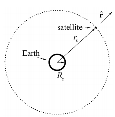
Choose the origin at the center of the earth, and the unit vector \(\hat{\mathbf{r}}\) along the radial direction. This choice of coordinates makes sense in this problem since the direction of acceleration is along the radial direction.

Let \(\overrightarrow{\mathbf{r}}\) be the position vector of the satellite. The magnitude of \(\overrightarrow{\mathbf{r}}\) (we denote it as \(r_{\mathrm{s}}\)) is the distance of the satellite from the center of the earth, and hence the radius of its circular orbit. Let ω be the angular velocity of the satellite, and the period is \(T=2 \pi / \omega\) The acceleration is directed inward, with magnitude \(r_{\mathrm{s}} \omega^{2}\); in vector form,

\[\overrightarrow{\mathbf{a}}=-r_{s} \omega^{2} \hat{\mathbf{r}} \nonumber \]

Apply Newton’s Second Law to the satellite for the radial component. The only force in this direction is the gravitational force due to the Earth,

\[\overrightarrow{\mathrm{F}}_{\mathrm{grav}}=-m_{\mathrm{s}} \omega^{2} r_{\mathrm{s}} \hat{\mathbf{r}} \nonumber \]

The inward radial force on the satellite is the gravitational attraction of the earth,

\[-G \frac{m_{\mathrm{s}} m_{\mathrm{e}}}{r_{\mathrm{s}}^{2}} \hat{\mathbf{r}}=-m_{\mathrm{s}} \omega^{2} r_{\mathrm{s}} \hat{\mathbf{r}} \nonumber \]

Equating the \(\hat{\mathbf{r}}\) components,

\[G \frac{m_{\mathrm{s}} m_{\mathrm{e}}}{r_{\mathrm{s}}^{2}}=m_{\mathrm{s}} \omega^{2} r_{\mathrm{s}} \nonumber \]

Solving for the radius of orbit of the satellite \(r_{\mathrm{s}}\),

\[r_{\mathrm{s}}=\left(\frac{G m_{\mathrm{e}}}{\omega^{2}}\right)^{1 / 3} \nonumber \]

The period T of the satellite’s orbit in seconds is 86164 s and so the angular speed is

\[\omega=\frac{2 \pi}{T}=\frac{2 \pi}{86164 \mathrm{s}}=7.2921 \times 10^{-5} \mathrm{s}^{-1} \nonumber \]

Using the values of ω, G and \(m_{\mathrm{e}}\) in Equation (9.3.5), we determine \(r_{\mathrm{s}}\),

\[r_{\mathrm{s}}=4.22 \times 10^{7} \mathrm{m}=6.62 \mathrm{R}_{\mathrm{e}} \nonumber \]

Example 9.2 Double Star System

Consider a double star system under the influence of gravitational force between the stars. Star 1 has mass \(m_{1}\) and star 2 has mass \(m_{2}\). Assume that each star undergoes uniform circular motion such that the stars are always a fixed distance s apart (rotating counterclockwise in Figure 9.5). What is the period of the orbit?

Figure 9.5 Two stars undergoing circular orbits about each other

Solution: Because the distance between the two stars doesn’t change as they orbit about each other, there is a central point where the lines connecting the two objects intersect as the objects move, as can be seen in the figure above. (We will see later on in the course that central point is the center of mass of the system.) Choose radial coordinates for each star with origin at that central point. Let \(\hat{\mathbf{r}}_{1}\) be a unit vector at Star 1 pointing radially away from the center of mass. The position of object 1 is then \(\overrightarrow{\mathbf{r}}_{1}=r_{1} \hat{\mathbf{r}}_{1}\), where \(r_{1}\) is the distance from the central point. Let \(\hat{\mathbf{r}}_{2}\) be a unit vector at Star 2 pointing radially away from the center of mass. The position of object 2 is then \(\overrightarrow{\mathbf{r}}_{2}=r_{2} \hat{\mathbf{r}}_{2}\), where \(r_{2}\) is the distance from the central point. Because the distance between the two stars is fixed we have that

\[s=r_{1}+r_{2} \nonumber \]

The coordinate system is shown in Figure 9.6

Figure 9.6 Coordinate system for double star orbits

The gravitational force on object 1 is then

\[\overrightarrow{\mathbf{F}}_{2,1}=-\frac{G m_{1} m_{2}}{s^{2}} \hat{\mathbf{r}}_{1} \nonumber \]

The gravitational force on object 2 is then

\[\overrightarrow{\mathbf{F}}_{1,2}=-\frac{G m_{1} m_{2}}{s^{2}} \hat{\mathbf{r}}_{2} \nonumber \]

The force diagrams on the two stars are shown in Figure 9.7.

Figure 9.7 Force diagrams on objects 1 and 2

Let ω denote the magnitude of the angular velocity of each star about the central point. Then Newton’s Second Law, \(\overrightarrow{\mathbf{F}}_{1}=m_{1} \overrightarrow{\mathbf{a}}_{1}\) for Star 1 in the radial direction \(\hat{\mathbf{r}}_{1}\) is

\[-G \frac{m_{1} m_{2}}{s^{2}}=-m_{1} r_{1} \omega^{2} \nonumber \]

We can solve this for \(r_{1}\),

\[r_{1}=G \frac{m_{2}}{\omega^{2} s^{2}} \nonumber \]

Newton’s Second Law, \(\overrightarrow{\mathbf{F}}_{2}=m_{2} \overrightarrow{\mathbf{a}}_{2}\) for Star 2 in the radial direction \(\hat{\mathbf{r}}_{2}\) is

\[-G \frac{m_{1} m_{2}}{s^{2}}=-m_{2} r_{2} \omega^{2} \nonumber \]

We can solve this for \(r_{2}\)

\[r_{2}=G \frac{m_{1}}{\omega^{2} s^{2}} \nonumber \]

Because s , the distance between the stars, is constant

\[s=r_{1}+r_{2}=G \frac{m_{2}}{\omega^{2} s^{2}}+G \frac{m_{1}}{\omega^{2} s^{2}}=G \frac{\left(m_{2}+m_{1}\right)}{\omega^{2} s^{2}} \nonumber \]

Thus the magnitude of the angular velocity is

\[\omega=\left(G \frac{\left(m_{2}+m_{1}\right)}{s^{3}}\right)^{1 / 2} \nonumber \]

and the period is then

\[T=\frac{2 \pi}{\omega}=\left(\frac{4 \pi^{2} s^{3}}{G\left(m_{2}+m_{1}\right)}\right)^{1 / 2} \nonumber \]

Note that both masses appear in the above expression for the period unlike the expression for Kepler’s Law for circular orbits. Equation (9.2.7). The reason is that in the argument leading up to Equation (9.2.7), we assumed that \(m_{1}<<m_{2}\), this was equivalent to assuming that the central point was located at the center of the Earth. If we used Equation (9.3.8) instead we would find that the orbital period for the circular motion of the Earth and moon about each other is

\[T=\sqrt{\frac{4 \pi^{2}\left(3.82 \times 10^{8} \mathrm{m}\right)^{3}}{\left(6.67 \times 10^{-11} \mathrm{N} \cdot \mathrm{m}^{2} \cdot \mathrm{kg}^{-2}\right)\left(5.98 \times 10^{24} \mathrm{kg}+7.36 \times 10^{22} \mathrm{kg}\right)}}=2.33 \times 10^{6} \mathrm{s} \nonumber \]

which is \(1.43 \times 10^{4} \mathrm{s}=0.17\)d shorter than our previous calculation.

Example 9.3 Rotating Objects

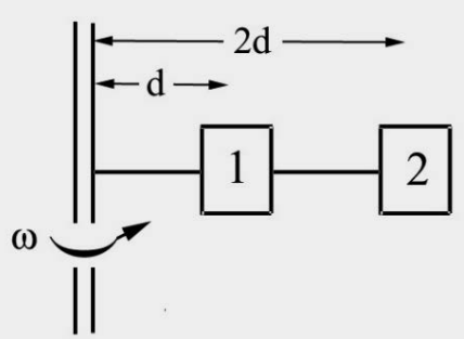
Two objects 1 and 2 of mass \(m_{1}\) and \(m_{2}\) are whirling around a shaft with a constant angular velocity ω . The first object is a distance d from the central axis, and the second object is a distance 2d from the axis (Figure 9.8). You may ignore the mass of the strings and neglect the effect of gravity. (a) What is the tension in the string between the inner object and the outer object? (b) What is the tension in the string between the shaft and the inner object?

Figure 9.8 Objects attached to a rotating shaft

Solution: We begin by drawing separate force diagrams, Figure 9.9a for object 1 and Figure 9.9b for object 2.

Figure 9.9 (a) and 9.9 (b) Free-body force diagrams for objects 1 and 2

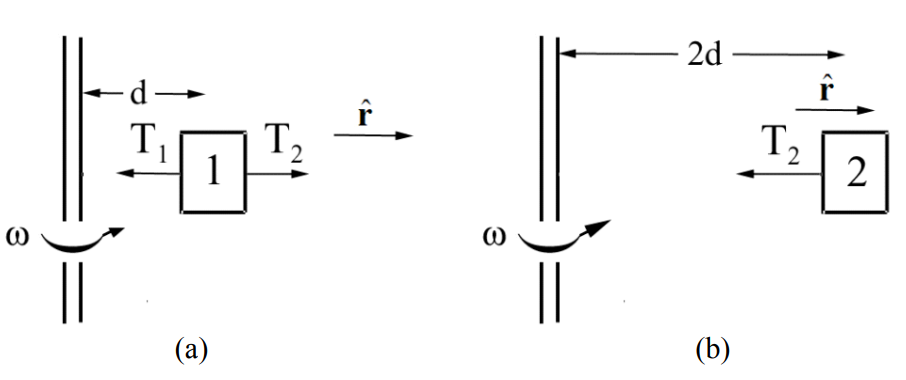
Newton’s Second Law, \(\overrightarrow{\mathbf{F}}_{1}=m_{1} \overrightarrow{\mathbf{a}}_{1}\), for the inner object in the radial direction is

\[\hat{\mathbf{r}}: T_{2}-T_{1}=-m_{1} d \omega^{2} \nonumber \]

Newton’s Second Law, \(\overrightarrow{\mathbf{F}}_{2}=m_{2} \overrightarrow{\mathbf{a}}_{2}\), for the outer object in the radial direction is

\[\hat{\mathbf{r}}:-T_{2}=-m_{2} 2 d \omega^{2} \nonumber \]

The tension in the string between the inner object and the outer object is therefore

\[T_{2}=m_{2} 2 d \omega^{2} \nonumber \]

Using this result for \(T_{2}\) in the force equation for the inner object yields

\[m_{2} 2 d \omega^{2}-T_{1}=-m_{1} d \omega^{2} \nonumber \]

which can be solved for the tension in the string between the shaft and the inner object

\[T_{1}=d \omega^{2}\left(m_{1}+2 m_{2}\right) \nonumber \]

Example 9.4 Tension in a Rope

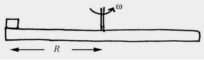
A uniform rope of mass mand length L is attached to shaft that is rotating at constant angular velocity ω . Find the tension in the rope as a function of distance from the shaft. You may ignore the effect of gravitation.

Solution: Divide the rope into small pieces of length \(\Delta r\), each of mass \(\Delta m=(m / L) \Delta r\) Consider the piece located a distance r from the shaft (Figure 9.10).

Figure 9.10 Small slice of rotating rope

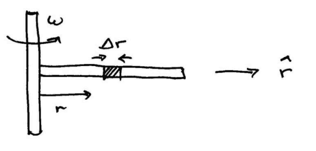
The radial component of the force on that piece is the difference between the tensions evaluated at the sides of the piece, \(F_{r}=T(r+\Delta r)-T(r)\), (Figure 9.11).

Figure 9.11 Free-body force diagram on small slice of rope

The piece is accelerating inward with a radial component \(a_{r}=-r \omega^{2}\). Thus Newton’s Second Law becomes

\[\begin{array}{l}
F_{r}=-\Delta m \omega^{2} r \\
T(r+\Delta r)-T(r)=-(m / L) \Delta r r \omega^{2}
\end{array} \nonumber \]

Denote the difference in the tension by \(\Delta T=T(r+\Delta r)-T(r)\). After dividing through by Δr , Equation (9.3.9) becomes

\[\frac{\Delta T}{\Delta r}=-(m / L) r \omega^{2} \nonumber \]

In the limit as \(\Delta r \rightarrow 0\), Equation (9.3.10) becomes a differential equation,

\[\frac{d T}{d r}=-(m / L) \omega^{2} r \nonumber \]

From this, we see immediately that the tension decreases with increasing radius. We shall solve this equation by integration

\[\begin{aligned}
T(r)-T(L) &=\int_{r^{\prime}=L}^{r^{\prime}=r} \frac{d T}{d r^{\prime}} d r^{\prime}=-\left(m \omega^{2} / L\right) \int_{L}^{r} r^{\prime} d r^{\prime} \\
&=-\left(m \omega^{2} / 2 L\right)\left(r^{2}-L^{2}\right) \\
&=\left(m \omega^{2} / 2 L\right)\left(L^{2}-r^{2}\right)
\end{aligned} \nonumber \]

We use the fact that the tension, in the ideal case, will vanish at the end of the rope, r = L . Thus,

\[T(r)=\left(m \omega^{2} / 2 L\right)\left(L^{2}-r^{2}\right) \nonumber \]

This last expression shows the expected functional form, in that the tension is largest closest to the shaft, and vanishes at the end of the rope.

Example 9.5 Object Sliding in a Circular Orbit on the Inside of a Cone

Consider an object of mass m that slides without friction on the inside of a cone moving in a circular orbit with constant speed \(v_{0}\). The cone makes an angle θ with respect to a vertical axis. The axis of the cone is vertical and gravity is directed downwards. The apex half-angle of the cone is θ as shown in Figure 9.12. Find the radius of the circular path and the time it takes to complete one circular orbit in terms of the given quantities and g .

Figure 9.12 Object in a circular orbit on inside of a cone

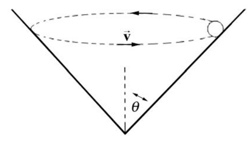
Solution: Choose cylindrical coordinates as shown in the above figure. Choose unit vectors \(\hat{\mathbf{r}}\) pointing in the radial outward direction and \(\hat{\mathbf{k}}\) pointing upwards. The force diagram on the object is shown in Figure 9.13.

Figure 9.13 Free-body force diagram on object

The two forces acting on the object are the normal force of the wall on the object and the gravitational force. Then Newton’s Second Law in the \(\hat{\mathbf{r}}\)-direction becomes

\[-N \cos \theta=\frac{-m v^{2}}{r} \nonumber \]

and in the \(\hat{\mathbf{k}}\)-direction becomes

\[N \sin \theta-m g=0 \nonumber \]

These equations can be re-expressed as

\(\begin{array}{l}
N \cos \theta=m \frac{v^{2}}{r} \\
N \sin \theta=m g
\end{array}\)

We can divide these two equations,

\(\frac{N \sin \theta}{N \cos \theta}=\frac{m g}{m v^{2} / r}\)

yielding

\(\tan \theta=\frac{r g}{v^{2}}\)

This can be solved for the radius,

\(r=\frac{v^{2}}{g} \tan \theta\)

The centripetal force in this problem is the vector component of the contact force that is pointing radially inwards,

\[F_{\text {cent }}=N \cos \theta=m g \cot \theta \nonumber \]

where \(N \sin \theta=m g\) has been used to eliminate N in terms of m , g and θ . The radius is independent of the mass because the component of the normal force in the vertical direction must balance the gravitational force, and so the normal force is proportional to the mass.

Example 9.6 Coin on a Rotating Turntable

A coin of mass m (which you may treat as a point object) lies on a turntable, exactly at the rim, a distance R from the center. The turntable turns at constant angular speed ω and the coin rides without slipping. Suppose the coefficient of static friction between the turntable and the coin is given by µ . Let g be the gravitational constant. What is the maximum angular speed \(\omega_{\max }\) such that the coin does not slip?

Figure 9.14 Coin on Rotating Turntable

Solution: The coin undergoes circular motion at constant speed so it is accelerating inward. The force inward is static friction and at the just slipping point it has reached its maximum value. We can use Newton’s Second Law to find the maximum angular speed \(\omega_{\max }\). We choose a polar coordinate system and the free-body force diagram is shown in the figure below.

Figure 9.15 Free-body force diagram on coin

The contact force is given by

\[\overrightarrow{\mathbf{C}}=\overrightarrow{\mathbf{N}}+\overrightarrow{\mathbf{f}}_{\mathrm{s}}=N \hat{\mathbf{k}}-f_{\mathrm{s}} \hat{\mathbf{r}} \nonumber \]

The gravitational force is given by

\[\overrightarrow{\mathbf{F}}_{g r a v}=-m g \hat{\mathbf{k}} \nonumber \]

Newton’s Second Law in the radial direction is given by

\[-f_{\mathrm{s}}=-m R \omega^{2} \nonumber \]

Newton’s Second Law, \(F_{z}=m a_{z}\) in the z-direction, noting that the disc is static hence \(a_{z}=0\), is given by

\[N-m g=0 \nonumber \]

Thus the normal force is

\[N=m g \nonumber \]

As ω increases, the static friction increases in magnitude until at \(\omega=\omega_{\max }\) and static friction reaches its maximum value (noting Equation (9.3.18)).

\[\left(f_{\mathrm{s}}\right)_{\max }=\mu N=\mu m g \nonumber \]

At this value the disc slips. Thus substituting this value for the maximum static friction into Equation (9.3.16) yields

\[\mu m g=m R \omega_{\max }^{2} \nonumber \]

We can now solve Equation (9.3.20) for maximum angular speed \(\omega_{\max }\) such that the coin does not slip

\[\omega_{\max }=\sqrt{\frac{\mu g}{R}} \nonumber \]