13.9: Work done by a Non-Constant Force Along an Arbitrary Path

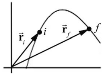
Suppose that a non-constant force \(\overrightarrow{\mathbf{F}}\) acts on a point-like body of mass m while the body is moving on a three dimensional curved path. The position vector of the body at time t with respect to a choice of origin is \(\overrightarrow{\mathbf{r}}(t)\). In Figure 13.15 we show the orbit of the body for a time interval \(\left[t_{i}, t_{f}\right]\) moving from an initial position \(\overrightarrow{\mathbf{r}}_{i} \equiv \overrightarrow{\mathbf{r}}\left(t=t_{i}\right)\) at time \(t=t_{i}\) to a final position \(\overrightarrow{\mathbf{r}}_{f} \equiv \overrightarrow{\mathbf{r}}\left(t=t_{f}\right)\) at time \(t=t_{f}\).

Figure 13.15 Path traced by the motion of a body.

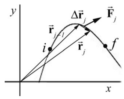
We divide the time interval \(\left[t_{i}, t_{f}\right]\) into N smaller intervals with \(\left[t_{j-1}, t_{j}\right]\), \(j=1, \cdots, N\) with \(t_{N}=t_{f}\). Consider two position vectors \(\overrightarrow{\mathbf{r}}_{j} \equiv \overrightarrow{\mathbf{r}}\left(t=t_{j}\right)\) and \(\overrightarrow{\mathbf{r}}_{j-1} \equiv \overrightarrow{\mathbf{r}}\left(t=t_{j-1}\right)\) the displacement vector during the corresponding time interval as \(\Delta \overrightarrow{\mathbf{r}}_{j}=\overrightarrow{\mathbf{r}}_{j}-\overrightarrow{\mathbf{r}}_{j-1}\). Let \(\overrightarrow{\mathbf{F}}\) denote the force acting on the body during the interval \(\left[t_{j-1}, t_{j}\right]\). The average force in this interval is \(\left(\overrightarrow{\mathbf{F}}_{j}\right)_{\mathrm{ave}}\) and the average work \(\Delta W_{j}\) done by the force during the time interval \(\left[t_{j-1}, t_{j}\right]\) is the scalar product between the average force vector and the displacement vector,

\[\Delta W_{j}=\left(\overrightarrow{\mathbf{F}}_{j}\right)_{\mathrm{ave}} \cdot \Delta \overrightarrow{\mathbf{r}}_{j} \nonumber \]

The force and the displacement vectors for the time interval \(\left[t_{j-1}, t_{j}\right]\) are shown in Figure 13.16 (note that the subscript “ave” on \(\left(\overrightarrow{\mathbf{F}}_{j}\right)_{\mathrm{ave}}\) has been suppressed).

Figure 13.16 An infinitesimal work element.

We calculate the work by adding these scalar contributions to the work for each interval \(\left[t_{j-1}, t_{j}\right]\), for j =1 to N ,

\[W_{N}=\sum_{j=1}^{j=N} \Delta W_{j}=\sum_{j=1}^{j=N}\left(\overrightarrow{\mathbf{F}}_{j}\right)_{\mathrm{ave}} \cdot \Delta \overrightarrow{\mathbf{r}}_{j} \nonumber \]

We would like to define work in a manner that is independent of the way we divide the interval, so we take the limit as \(N \rightarrow \infty\) and \(\left|\Delta \overrightarrow{\mathbf{r}}_{j}\right| \rightarrow 0\) for all j . In this limit, as the intervals become smaller and smaller, the distinction between the average force and the actual force vanishes. Thus if this limit exists and is well defined, then the work done by the force is

\[W=\lim _{N \rightarrow \infty \atop\left|\Delta \overrightarrow{\mathbf{r}}_{j}\right| \rightarrow 0} \sum_{j=1}^{j=N}\left(\overrightarrow{\mathbf{F}}_{j}\right)_{\text {ave }} \cdot \Delta \overrightarrow{\mathbf{r}}_{j}=\int_{i}^{f} \overrightarrow{\mathbf{F}} \cdot d \overrightarrow{\mathbf{r}} \nonumber \]

Notice that this summation involves adding scalar quantities. This limit is called the line integral of the force \(\overrightarrow{\mathbf{F}}\). The symbol \(d \overrightarrow{\mathbf{r}}\) is called the infinitesimal vector line element. At time t, \(d \overrightarrow{\mathbf{r}}\) is tangent to the orbit of the body and is the limit of the displacement vector \(\Delta \overrightarrow{\mathbf{r}}=\overrightarrow{\mathbf{r}}(t+\Delta t)-\overrightarrow{\mathbf{r}}(t)\) as Δt approaches zero. In this limit, the parameter t does not appear in the expression in Equation (13.8.19).

In general this line integral depends on the particular path the body takes between the initial position \(\overrightarrow{\mathbf{r}}_{i}\) and the final position \(\overrightarrow{\mathbf{r}}_{f}\), which matters when the force \(\overrightarrow{\mathbf{F}}\) is nonconstant in space, and when the contribution to the work can vary over different paths in space. We can represent the integral in Equation (13.8.19) explicitly in a coordinate system by specifying the infinitesimal vector line element d\(\overrightarrow{\mathbf{r}}\) and then explicitly computing the scalar product.

Work Integral in Cartesian Coordinates

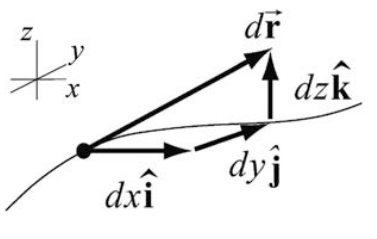
In Cartesian coordinates the line element is

\[d \overrightarrow{\mathbf{r}}=d x \hat{\mathbf{i}}+d y \hat{\mathbf{j}}+d z \hat{\mathbf{k}} \nonumber \]

where dx , dy , and dz represent arbitrary displacements in the \(\hat{\mathbf{i}}-, \hat{\mathbf{j}}-\), and \(\hat{\mathbf{k}}\)-direction respectively as seen in Figure 13.17.

Figure 13.17 A line element in Cartesian coordinates.

The force vector can be represented in vector notation by

\[\overrightarrow{\mathbf{F}}=F_{x} \hat{\mathbf{i}}+F_{y} \hat{\mathbf{j}}+F_{z} \hat{\mathbf{k}} \nonumber \]

The infinitesimal work is the sum of the work done by the component of the force times the component of the displacement in each direction,

\[d W=F_{x} d x+F_{y} d y+F_{z} d z \nonumber \]

Equation (13.8.22) is just the scalar product

\[\begin{aligned}
d W &=\overrightarrow{\mathbf{F}} \cdot d \overrightarrow{\mathbf{r}}=\left(F_{x} \hat{\mathbf{i}}+F_{y} \hat{\mathbf{j}}+F_{z} \hat{\mathbf{k}}\right) \cdot(d x \hat{\mathbf{i}}+d y \hat{\mathbf{j}}+d z \hat{\mathbf{k}}) \\
&=F_{x} d x+F_{y} d y+F_{z} d z
\end{aligned} \nonumber \]

The work is

\[W=\int_{\overrightarrow{\mathbf{r}}=\overrightarrow{\mathbf{r}}_{0}}^{\overrightarrow{\mathbf{r}}=\overrightarrow{\mathbf{r}}_{f}} \overrightarrow{\mathbf{F}} \cdot d \overrightarrow{\mathbf{r}}=\int_{\overrightarrow{\mathbf{r}}=\overrightarrow{\mathbf{r}}_{0}}^{\overrightarrow{\mathbf{r}}=\overrightarrow{\mathbf{r}}_{f}}\left(F_{x} d x+F_{y} d y+F_{z} d z\right)=\int_{\overrightarrow{\mathbf{r}}=\overrightarrow{\mathbf{r}}_{0}}^{\overrightarrow{\mathbf{r}}=\overrightarrow{\mathbf{r}}_{f}} F_{x} d x+\int_{\overrightarrow{\mathbf{r}}=\overrightarrow{\mathbf{r}}_{0}}^{\overrightarrow{\mathbf{r}}=\overrightarrow{\mathbf{r}}_{f}} \cdot \overrightarrow{d y+\int_{z=\overrightarrow{\mathbf{r}}_{0}}} F_{z} d z \nonumber \]

Work Integral in Cylindrical Coordinates

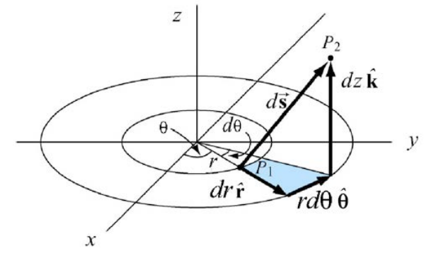
In cylindrical coordinates the line element is

\[d \overrightarrow{\mathbf{r}}=d r \hat{\mathbf{r}}+r d \theta \hat{\mathbf{\theta}}+d z \hat{\mathbf{k}} \nonumber \]

where dr , rdθ , and dz represent arbitrary displacements in the \(\hat{\mathbf{r}}-, \hat{\boldsymbol{\theta}}-\) and \(\hat{\mathbf{k}}-\) directions respectively as seen in Figure 13.18.

Figure 13.18 Displacement vector \(d \overrightarrow{\mathbf{s}}\) between two points

The force vector can be represented in vector notation by

\[\overrightarrow{\mathbf{F}}=F_{r} \hat{\mathbf{r}}+F_{\theta} \hat{\boldsymbol{\theta}}+F_{z} \hat{\mathbf{k}} \nonumber \]

The infinitesimal work is the scalar product

\[\begin{aligned}
d W &=\overrightarrow{\mathbf{F}} \cdot d \overrightarrow{\mathbf{r}}=\left(F_{r} \hat{\mathbf{r}}+F_{\theta} \hat{\boldsymbol{\theta}}+F_{z} \hat{\mathbf{k}}\right) \cdot(d r \hat{\mathbf{r}}+r d \theta \hat{\boldsymbol{\theta}}+d z \hat{\mathbf{k}}) \\
&=F_{r} d r+F_{\theta} r d \theta+F_{z} d z
\end{aligned} \nonumber \]

The work is

\[W=\int_{\overrightarrow{\mathbf{r}}=\overrightarrow{\mathbf{r}}_{0}}^{\overrightarrow{\mathbf{r}}=\overrightarrow{\mathbf{r}}_{f}} \cdot \overrightarrow{\mathbf{r}}=\int_{\overrightarrow{\mathbf{r}}=\overrightarrow{\mathbf{r}}_{0}}^{\overrightarrow{\mathbf{r}}=\overrightarrow{\mathbf{r}}_{f}}\left(F_{r} d r+F_{\theta} r d \theta+F_{z} d z\right)=\int_{\overrightarrow{\mathbf{r}}=\overrightarrow{\mathbf{r}}_{0}}^{\overrightarrow{\mathbf{r}}=\overrightarrow{\mathbf{r}}_{f}} F_{r} d r+\int_{\overrightarrow{\mathbf{r}}=\overrightarrow{\mathbf{r}}_{0}}^{\overrightarrow{\mathbf{r}}=\overrightarrow{\mathbf{r}}_{f}} F_{\theta} r d \theta+\int_{\overrightarrow{\mathbf{r}}=\overrightarrow{\mathbf{r}}_{0}}^{\overrightarrow{\mathbf{r}}=\overrightarrow{\mathbf{r}}_{f}} F_{z} d z \nonumber \]