
17.4: Torque, Angular Acceleration, and Moment of Inertia
- Page ID
- 24532

Torque Equation for Fixed Axis Rotation
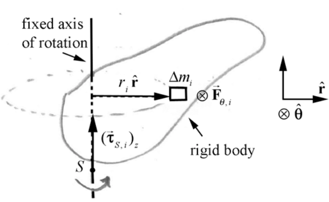
For fixed-axis rotation, there is a direct relation between the component of the torque along the axis of rotation and angular acceleration. Consider the forces that act on the rotating body. Generally, the forces on different volume elements will be different, and so we will denote the force on the volume element of mass \(\Delta m_{i}\) by \(\overrightarrow{\mathbf{F}}_{i}\). Choose the z - axis to lie along the axis of rotation. Divide the body into volume elements of mass \(\Delta m_{i}\). Let the point \(S\) denote a specific point along the axis of rotation (Figure 17.19). Each volume element undergoes a tangential acceleration as the volume element moves in a circular orbit of radius \(r_{i}=\left|\overrightarrow{\mathbf{r}}_{i}\right|\) about the fixed axis.

The vector from the point \(S\) to the volume element is given by
\[\overrightarrow{\mathbf{r}}_{S, i}=z_{i} \hat{\mathbf{k}}+\overrightarrow{\mathbf{r}}_{i}=z_{i} \hat{\mathbf{k}}+r_{i} \hat{\mathbf{r}} \nonumber \]
where \(z_{i}\) is the distance along the axis of rotation between the point \(S\) and the volume element. The torque about \(S\) due to the force \(\overrightarrow{\mathbf{F}}_{i}\) acting on the volume element is given by
\[\vec{\tau}_{S, i}=\overrightarrow{\mathbf{r}}_{S, i} \times \overrightarrow{\mathbf{F}}_{i} \nonumber \]
Substituting Equation (17.3.1) into Equation (17.3.2) gives
\[\vec{\tau}_{S, i}=\left(z_{i} \hat{\mathbf{k}}+r_{i} \hat{\mathbf{r}}\right) \times \overrightarrow{\mathbf{F}}_{i} \nonumber \]
For fixed-axis rotation, we are interested in the z -component of the torque, which must be the term
\[\left(\vec{\tau}_{S, i}\right)_{z}=\left(r_{i} \hat{\mathbf{r}} \times \overrightarrow{\mathbf{F}}_{i}\right)_{z} \nonumber \]
because the vector product \(z_{i} \hat{\mathbf{k}} \times \overrightarrow{\mathbf{F}}_{i}\) must be directed perpendicular to the plane formed by the vectors \(\hat{\mathbf{k}}\) and \(\overrightarrow{\mathbf{F}}_{i}\), hence perpendicular to the z -axis. The force acting on the volume element has components
\[\overrightarrow{\mathbf{F}}_{i}=F_{r, i} \hat{\mathbf{r}}+F_{\theta, i} \hat{\boldsymbol{\theta}}+F_{z, i} \hat{\mathbf{k}} \nonumber \]
The z -component \(F_{z, i}\) of the force cannot contribute a torque in the z -direction, and so substituting Equation (17.3.5) into Equation (17.3.4) yields
\[\left(\vec{\tau}_{S, i}\right)_{z}=\left(r_{i} \hat{\mathbf{r}} \times\left(F_{r, i} \hat{\mathbf{r}}+F_{\theta, i} \hat{\boldsymbol{\theta}}\right)\right)_{z} \nonumber \]
The radial force does not contribute to the torque about the z -axis, since
\[r_{i} \hat{\mathbf{r}} \times F_{r, i} \hat{\mathbf{r}}=\overrightarrow{\mathbf{0}} \nonumber \]
So, we are interested in the contribution due to torque about the z -axis due to the tangential component of the force on the volume element (Figure 17.20). The component of the torque about the z -axis is given by
\[\left(\vec{\tau}_{S, i}\right)_{z}=\left(r_{i} \hat{\mathbf{r}} \times F_{\theta, i} \hat{\mathbf{\theta}}\right)_{z}=r_{i} F_{\theta, i} \nonumber \]
The z -component of the torque is directed upwards in Figure 17.20, where \(F_{\theta, i}\) is positive (the tangential force is directed counterclockwise, as in the figure). Applying Newton’s Second Law in the tangential direction,
\[F_{\theta, i}=\Delta m_{i} a_{\theta, i} \nonumber \]
Using our kinematics result that the tangential acceleration is \(a_{\theta, i}=r_{i} \alpha_{z}\), where \(\alpha_{z}\) is the z -component of angular acceleration, we have that
\[F_{\theta, i}=\Delta m_{i} r_{i} \alpha_{z} \nonumber \]
From Equation (17.3.8), the component of the torque about the z -axis is then given by
\[\left(\vec{\tau}_{S, i}\right)_{z}=r_{i} F_{\theta, i}=\Delta m_{i} r_{i}^{2} \alpha_{z} \nonumber \]
The component of the torque about the z -axis is the summation of the torques on all the volume elements,
\[\begin{aligned}
\left(\vec{\tau}_{S}\right)_{z} &=\sum_{i=1}^{i=N}\left(\vec{\tau}_{S, i}\right)_{z}=\sum_{i=1}^{i=N} r_{\perp, i} F_{\theta, i} \\
&=\sum_{i=1}^{i=N} \Delta m_{i} r_{i}^{2} \alpha_{z}
\end{aligned} \nonumber \]
Because each element has the same z -component of angular acceleration, \(\alpha_{z}\), the summation becomes
\[\left(\vec{\tau}_{S}\right)_{z}=\left(\sum_{i=1}^{i=N} \Delta m_{i} r_{i}^{2}\right) \alpha_{z} \nonumber \]
Recalling our definition of the moment of inertia, (Chapter 16.3) the z -component of the torque is proportional to the z -component of angular acceleration,
\[\tau_{S, z}=I_{S} \alpha_{z} \nonumber \]
and the moment of inertia, \(I_{S}\), is the constant of proportionality. The torque about the point \(S\) is the sum of the external torques and the internal torques
\[\vec{\tau}_{S}=\vec{\tau}_{S}^{\mathrm{ext}}+\vec{\tau}_{S}^{\mathrm{int}} \nonumber \]
The external torque about the point \(S\) is the sum of the torques due to the net external force acting on each element
\[\vec{\tau}_{S}^{\mathrm{ext}}=\sum_{i=1}^{i=N} \vec{\tau}_{S, i}^{\mathrm{ext}}=\sum_{i=1}^{i=N} \overrightarrow{\mathbf{r}}_{S, i} \times \overrightarrow{\mathbf{F}}_{i}^{\mathrm{ext}} \nonumber \]
The internal torque arise from the torques due to the internal forces acting between pairs of elements
\[\vec{\tau}_{S}^{\mathrm{int}}=\sum_{i=1}^{N} \vec{\tau}_{S, j}^{\mathrm{int}}=\sum_{i=1}^{i=N} \sum_{j=1 \atop j \neq i}^{j=N} \vec{\tau}_{S, j, i}^{\mathrm{int}}=\sum_{i=1}^{i=N} \sum_{j=1 \atop j \neq i}^{j=N} \overrightarrow{\mathbf{r}}_{S, i} \times \overrightarrow{\mathbf{F}}_{j, i} \nonumber \]
We know by Newton’s Third Law that the internal forces cancel in pairs, \(\overrightarrow{\mathbf{F}}_{j, i}=-\overrightarrow{\mathbf{F}}_{i, j}\), and hence the sum of the internal forces is zero
\[\overrightarrow{\mathbf{0}}=\sum_{i=1}^{i=N} \sum_{j=1 \atop j \neq i}^{j=N} \overrightarrow{\mathbf{F}}_{j, i} \nonumber \]
Does the same statement hold about pairs of internal torques? Consider the sum of internal torques arising from the interaction between the \(i^{t h}\) and \(j^{t h}\) particles
\[\vec{\tau}_{S, j, i}^{\mathrm{int}}+\vec{\tau}_{S, i, j}^{\mathrm{int}}=\overrightarrow{\mathbf{r}}_{S, i} \times \overrightarrow{\mathbf{F}}_{j, i}+\overrightarrow{\mathbf{r}}_{S, j} \times \overrightarrow{\mathbf{F}}_{i, j} \nonumber \]
By the Newton’s Third Law this sum becomes
\[\vec{\tau}_{S, j, i}^{\mathrm{int}}+\vec{\tau}_{S, i, j}^{\mathrm{int}}=\left(\overrightarrow{\mathrm{r}}_{S, i}-\overrightarrow{\mathbf{r}}_{S, j}\right) \times \overrightarrow{\mathbf{F}}_{j, i} \nonumber \]
In the Figure 17.21, the vector \(\overrightarrow{\mathbf{r}}_{S, i}-\overrightarrow{\mathbf{r}}_{S, j}\) points from the \(j^{t h}\) element to the \(i^{t h}\) element. If the internal forces between a pair of particles are directed along the line joining the two particles then the torque due to the internal forces cancel in pairs.
\[\vec{\tau}_{S, j, i}^{\mathrm{int}}+\vec{\tau}_{S, i, j}^{\mathrm{int}}=\left(\overrightarrow{\mathbf{r}}_{S, i}-\overrightarrow{\mathbf{r}}_{S, j}\right) \times \overrightarrow{\mathbf{F}}_{j, i}=\overrightarrow{\mathbf{0}} \nonumber \]

This is a stronger version of Newton’s Third Law than we have so far since we have added the additional requirement regarding the direction of all the internal forces between pairs of particles. With this assumption, the torque is just due to the external forces
\(\vec{\tau}_{S}=\vec{\tau}_{S}^{\mathrm{ext}}\)
Thus Equation (17.3.14) becomes
\(\left(\tau_{S}^{\mathrm{ext}}\right)_{z}=I_{S} \alpha_{z}\)
This is very similar to Newton’s Second Law: the total force is proportional to the acceleration,
\[\overrightarrow{\mathbf{F}}=m \overrightarrow{\mathbf{a}} \nonumber \]
where the mass, m, is the constant of proportionality.
Torque Acts at the Center of Gravity
Suppose a rigid body in static equilibrium consists of N particles labeled by the index \(i=1,2,3, \ldots, N\). Choose a coordinate system with a choice of origin O such that mass \(m_{i}\) has position \(\overrightarrow{\mathbf{r}}_{i}\). Each point particle experiences a gravitational force \(\overrightarrow{\mathbf{F}}_{\text {gravity }, i}=m_{i} \overrightarrow{\mathbf{g}}\). The total torque about the origin is then zero (static equilibrium condition),
\[\vec{\tau}_{O}=\sum_{i=1}^{i=N} \vec{\tau}_{O, i}=\sum_{i=1}^{i=N} \overrightarrow{\mathbf{r}}_{i} \times \overrightarrow{\mathbf{F}}_{\mathrm{gavity}, i}=\sum_{i=1}^{i=N} \overrightarrow{\mathbf{r}}_{i} \times m_{i} \overrightarrow{\mathrm{g}}=\overrightarrow{\mathbf{0}} \nonumber \]
If the gravitational acceleration \(\overrightarrow{\mathbf{g}}\) is assumed constant, we can rearrange the summation in Equation (17.3.25) by pulling the constant vector \(\overrightarrow{\mathbf{g}}\) out of the summation ( \(\overrightarrow{\mathbf{g}}\) appears in each term in the summation),
\[\vec{\tau}_{O}=\sum_{i=1}^{i=N} \overrightarrow{\mathbf{r}}_{i} \times m_{i} \overrightarrow{\mathbf{g}}=\left(\sum_{i=1}^{i=N} m_{i} \overrightarrow{\mathbf{r}}_{i}\right) \times \overrightarrow{\mathbf{g}}=\overrightarrow{\mathbf{0}} \nonumber \]
We now use our definition of the center of the center of mass, Equation (10.5.3), to rewrite Equation (17.3.26) as
\[\vec{\tau}_{O}=\sum_{i=1}^{i=N} \overrightarrow{\mathbf{r}}_{i} \times m_{i} \overrightarrow{\mathbf{g}}=M_{\mathrm{T}} \overrightarrow{\mathbf{R}}_{\mathrm{cm}} \times \overrightarrow{\mathbf{g}}=\overrightarrow{\mathbf{R}}_{\mathrm{cm}} \times M_{\mathrm{T}} \overrightarrow{\mathbf{g}}=\overrightarrow{\mathbf{0}} \nonumber \]
Thus the torque due to the gravitational force acting on each point-like particle is equivalent to the torque due to the gravitational force acting on a point-like particle of mass \(M_{\mathrm{T}}\) located at a point in the body called the center of gravity, which is equal to the center of mass of the body in the typical case in which the gravitational acceleration \(\overrightarrow{\mathbf{g}}\) is constant throughout the body.
Example 17.9 Turntable
The turntable in Example 16.1, of mass 1.2 kg and radius \(1.3 \times 10^{1}\) cm, has a moment of inertia \(I_{S}=1.01 \times 10^{-2} \mathrm{kg} \cdot \mathrm{m}^{2}\) about an axis through the center of the turntable and perpendicular to the turntable. The turntable is spinning at an initial constant frequency \(f_{i}=33 \text { cycles } \cdot \min ^{-1}\). The motor is turned off and the turntable slows to a stop in 8.0 s due to frictional torque. Assume that the angular acceleration is constant. What is the magnitude of the frictional torque acting on the turntable?
Solution: We have already calculated the angular acceleration of the turntable in Example 16.1, where we found that
\[\alpha_{z}=\frac{\Delta \omega_{z}}{\Delta t}=\frac{\omega_{f}-\omega_{i}}{t_{f}-t_{i}}=\frac{-3.5 \mathrm{rad} \cdot \mathrm{s}^{-1}}{8.0 \mathrm{s}}=-4.3 \times 10^{-1} \mathrm{rad} \cdot \mathrm{s}^{-2} \nonumber \]
and so the magnitude of the frictional torque is
\[\begin{aligned}
\left|\tau_{z}^{\text {fic }}\right| &=I_{S}\left|\alpha_{z}\right|=\left(1.01 \times 10^{-2} \mathrm{kg} \cdot \mathrm{m}^{2}\right)\left(4.3 \times 10^{-1} \mathrm{rad} \cdot \mathrm{s}^{-2}\right) \\
&=4.3 \times 10^{-3} \mathrm{N} \cdot \mathrm{m}
\end{aligned} \nonumber \]
Example 17.10 Pulley and blocks
A pulley of mass \(m_{\mathrm{p}}\), radius R , and moment of inertia about its center of mass \(I_{\mathrm{cm}}\), is attached to the edge of a table. An inextensible string of negligible mass is wrapped around the pulley and attached on one end to block 1 that hangs over the edge of the table (Figure 17.22). The other end of the string is attached to block 2 that slides along a table.
The coefficient of sliding friction between the table and the block 2 is \(\mu_{k}\). Block 1 has mass \(m_{1}\) and block 2 has mass \(m_{2}\), with \(m_{1}>\mu_{k} m_{2}\). At time t = 0 , the blocks are released from rest and the string does not slip around the pulley. At time \(t=t_{1}\) block 1 hits the ground. Let g denote the gravitational constant. (a) Find the magnitude of the acceleration of each block. (b) How far did the block 1 fall before hitting the ground?
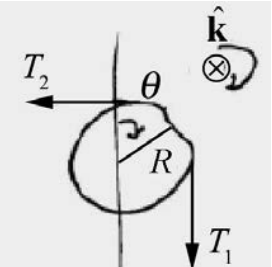
Solution: The torque diagram for the pulley is shown in the figure below where we choose \(\hat{\mathbf{k}}\) pointing into the page. Note that the tensions in the string on either side of the pulley are not equal. The reason is that the pulley is massive. To understand why, remember that the difference in the magnitudes of the torques due to the tension on either side of the pulley is equal to the moment of inertia times the magnitude of the angular acceleration, which is non -zero for a massive pulley. So the tensions cannot be equal. From our torque diagram, the torque about the point O at the center of the pulley is given by
\[\vec{\tau}_{O}=\overrightarrow{\mathbf{r}}_{O, 1} \times \overrightarrow{\mathbf{T}}_{1}+\overrightarrow{\mathbf{r}}_{O, 2} \times \overrightarrow{\mathbf{T}}_{2}=R\left(T_{1}-T_{2}\right) \hat{\mathbf{k}} \nonumber \]
Therefore the torque equation (17.3.23) becomes
\[R\left(T_{1}-T_{2}\right)=I_{z} \alpha_{z} \nonumber \]
The free body force diagrams on the two blocks are shown in Figure 17.23.

Newton’s Second Law on block 1 yields
\[m_{1} g-T_{1}=m_{1} a_{y 1} \nonumber \]
Newton’s Second Law on block 2 in the \(\hat{\mathbf{j}}\) direction yields
\[N-m_{2} g=0 \nonumber \]
Newton’s Second Law on block 2 in the \(\hat{\mathbf{i}}\) direction yields
\[T_{2}-f_{k}=m_{2} a_{x 2} \nonumber \]
The kinetic friction force is given by
\[f_{k}=\mu_{k} N=\mu_{k} m_{2} g \nonumber \]
Therefore Equation (17.3.34) becomes
\[T_{2}-\mu_{k} m_{2} g=m_{2} a_{x 2} \nonumber \]
Block 1 and block 2 are constrained to have the same acceleration so
\[a \equiv a_{x 1}=a_{x 2} \nonumber \]
We can solve Equations (17.3.32) and (17.3.36) for the two tensions yielding
\[T_{1}=m_{1} g-m_{1} a \nonumber \]
\[T_{2}=\mu_{k} m_{2} g+m_{2} a \nonumber \]
At point on the rim of the pulley has a tangential acceleration that is equal to the acceleration of the blocks so
\[a=a_{\theta}=R \alpha_{z} \nonumber \]
The torque equation (Equation (17.3.31)) then becomes
\[T_{1}-T_{2}=\frac{I_{z}}{R^{2}} a \nonumber \]
Substituting Equations (17.3.38) and (17.3.39) into Equation (17.3.41) yields
\[m_{1} g-m_{1} a-\left(\mu_{k} m_{2} g+m_{2} a\right)=\frac{I_{z}}{R^{2}} a \nonumber \]
which we can now solve for the accelerations of the blocks
\[a=\frac{m_{1} g-\mu_{k} m_{2} g}{m_{1}+m_{2}+I_{z} / R^{2}} \nonumber \]
Block 1 hits the ground at time \(t_{1}\), therefore it traveled a distance
\[y_{1}=\frac{1}{2}\left(\frac{m_{1} g-\mu_{k} m_{2} g}{m_{1}+m_{2}+I_{z} / R^{2}}\right) t_{1}^{2} \nonumber \]
Example 17.11 Experimental Method for Determining Moment of Inertia
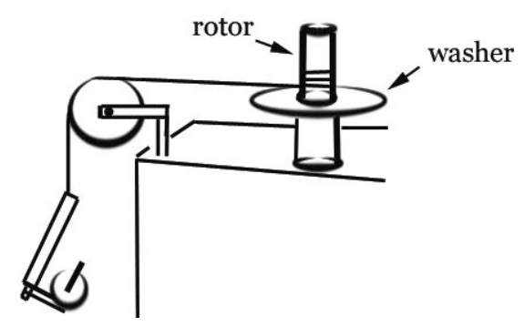
A steel washer is mounted on a cylindrical rotor of radius r =12.7 mm. A massless string, with an object of mass m = 0.055 kg attached to the other end, is wrapped around the side of the rotor and passes over a massless pulley (Figure 17.24). Assume that there is a constant frictional torque about the axis of the rotor. The object is released and falls. As the object falls, the rotor undergoes an angular acceleration of magnitude \(\alpha_{1}\). After the string detaches from the rotor, the rotor coasts to a stop with an angular acceleration of magnitude \(\alpha_{2}\). Let \(g=9.8 \mathrm{m} \cdot \mathrm{s}^{-2}\) denote the gravitational constant. Based on the data in the Figure 17.25, what is the moment of inertia \(I_{R}\) of the rotor assembly (including the washer) about the rotation axis?

Solution: We begin by drawing a force-torque diagram (Figure 17.26a) for the rotor and a free-body diagram for hanger (Figure 17.26b). (The choice of positive directions are indicated on the figures.) The frictional torque on the rotor is then given by \(\vec{\tau}_{f}=-\tau_{f} \hat{\mathbf{k}}\) where we use \(\tau_{f}\) as the magnitude of the frictional torque. The torque about the center of the rotor due to the tension in the string is given by \(\vec{\tau}_{T}=r T \hat{\mathbf{k}}\) where r is the radius of the rotor. The angular acceleration of the rotor is given by \(\vec{\alpha}_{1}=\alpha_{1} \hat{\mathbf{k}}\) and we expect that \(\alpha_{1}>0\) because the rotor is speeding up.
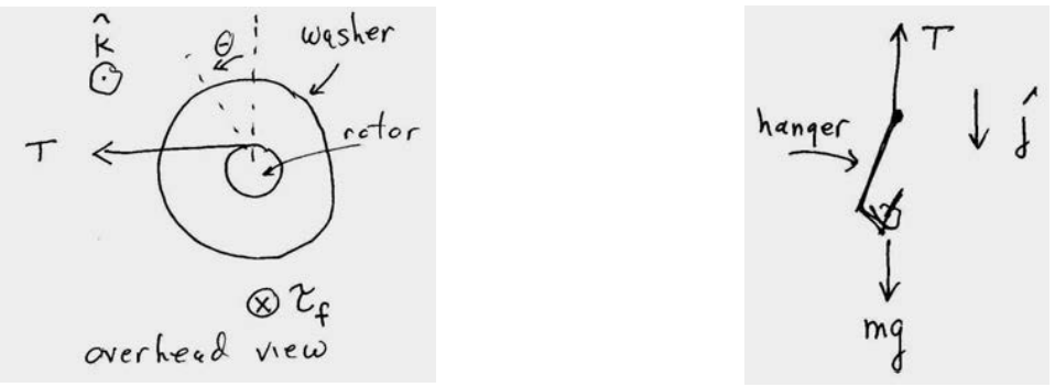
(a) (b)
Figure 17.26 (a) Force-torque diagram on rotor and (b) free-body force diagram on hanging object
While the hanger is falling, the rotor-washer combination has a net torque due to the tension in the string and the frictional torque, and using the rotational equation of motion,
\[\operatorname{Tr}-\tau_{f}=I_{R} \alpha_{1} \nonumber \]
We apply Newton’s Second Law to the hanger and find that
\[m g-T=m a_{1}=m \alpha_{1} r \nonumber \]
where \(a_{1}=r \alpha_{1}\) has been used to express the linear acceleration of the falling hanger to the angular acceleration of the rotor; that is, the string does not stretch. Before proceeding, it might be illustrative to multiply Equation (17.4.2) by r and add to Equation (17.4.1) to obtain
\[m g r-\tau_{f}=\left(I_{R}+m r^{2}\right) \alpha_{1} \nonumber \]
Equation (17.4.3) contains the unknown frictional torque, and this torque is determined by considering the slowing of the rotor/washer after the string has detached.

The torque on the system is just this frictional torque (Figure 17.27), and so
\[-\tau_{f}=I_{R} \alpha_{2} \nonumber \]
Note that in Equation (17.4.4), \(\tau_{f}>0\) and \(\alpha_{2}<0\). Subtracting Equation (17.4.4) from Equation (17.4.3) eliminates \(\tau_{f}\),
\[m g r=m r^{2} \alpha_{1}+I_{R}\left(\alpha_{1}-\alpha_{2}\right) \nonumber \]
We can now solve for \(I_{R}\) yielding
\[I_{R}=\frac{m r\left(g-r \alpha_{1}\right)}{\alpha_{1}-\alpha_{2}} \nonumber \]
For a numerical result, we use the data collected during a trial run resulting in the graph of angular speed vs. time for the falling object shown in Figure 17.25. The values for \(\alpha_{1}\) and \(\alpha_{2}\) can be determined by calculating the slope of the two straight lines in Figure 17.28 yielding
\[\begin{array}{l}
\alpha_{1}=\left(96 \mathrm{rad} \cdot \mathrm{s}^{-1}\right) /(1.15 \mathrm{s})=83 \mathrm{rad} \cdot \mathrm{s}^{-2} \\
\alpha_{2}=-\left(89 \mathrm{rad} \cdot \mathrm{s}^{-1}\right) /(2.85 \mathrm{s})=-31 \mathrm{rad} \cdot \mathrm{s}^{-2}
\end{array} \nonumber \]
Inserting these values into Equation (17.4.6) yields
\[I_{R}=5.3 \times 10^{-5} \mathrm{kg} \cdot \mathrm{m}^{2} \nonumber \]