
28.2: Velocity Vector Field
- Page ID
- 25564

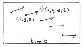
When we describe the flow of a fluid like water, we may think of the movement of individual particles. These particles interact with each other through forces. We could then apply our laws of motion to each individual particle in the fluid but because the number of particles is very large, this would be an extremely difficult computation problem. Instead we shall begin by mathematically describing the state of moving fluid by specifying the velocity of the fluid at each point in space and at each instant in time. For the moment we will choose Cartesian coordinates and refer to the coordinates of a point in space by the ordered triple (x, y, z) and the variable t to describe the instant in time, but in principle we may chose any appropriate coordinate system appropriate for describing the motion. The distribution of fluid velocities is described by the vector function v(x, y,z,t) . This represents the velocity of the fluid at the point (x, y, z) at the instant t . The quantity v(x, y,z,t) is called the velocity vector field. It can be thought of at each instant in time as a collection of vectors, one for each point in space whose direction and magnitude describes the direction and magnitude of the velocity of the fluid at that point (Figure 28.1). This description of the velocity vector field of the fluid refers to fixed points in space and not to moving particles in the fluid.
We shall introduce functions for the pressure P(x, y, z, t) and the density \(\rho(x, y, z, t)\) of the fluid that describe the pressure and density of the fluid at each point in space and at each instant in time. These functions are called scalar fields because there is only one number with appropriate units associated with each point in space at each instant in time.
In order to describe the velocity vector field completely we need three functions \(v_{x}(x, y, z, t), v_{y}(x, y, z, t), \text { and } v_{z}(x, y, z, t)\) to describe the components of the velocity vector field.
\[\overrightarrow{\mathbf{v}}(x, y, z, t)=v_{x}(x, y, z, t) \hat{\mathbf{i}}+v_{y}(x, y, z, t) \hat{\mathbf{j}}+v_{z}(x, y, z, t) \hat{\mathbf{k}}\end{equation}
The three component functions are scalar fields. The velocity vector field is in general quite complicated for a three-dimensional time dependent flow. We can sometimes make some simplifying assumptions that enable us to model a complex flow, for example modeling the flow as a two-dimensional flow or even further assumptions that one component function of a two-dimensional flow is negligible allowing us to model the flow as one-dimensional. For most flows, the velocity field varies in time. For some special cases we can model the flow by assuming that the velocity field does not change in time, a case we shall refer to as steady flow,
\[\frac{\partial \overrightarrow{\mathbf{v}}(x, y, z, t)}{\partial t}=\overrightarrow{\mathbf{0}} \quad(\text { steady flow }) \nonumber \]
For steady flows the velocity field is independent of time,
\[\overrightarrow{\mathbf{v}}(x, y, z)=v_{x}(x, y, z) \hat{\mathbf{i}}+v_{y}(x, y, z) \hat{\mathbf{j}}+v_{z}(x, y, z) \hat{\mathbf{k}} \quad(\text { steady flow }) \nonumber \]
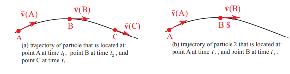
Let’s trace the motion of particles in an ideal fluid undergoing steady flow during a succession of intervals of duration \(\Delta t\) Consider particle 1 located at point A with coordinates \(\left(x_{A}, y_{A}, z_{A}\right)\). At the instant \(t_{1}\) particle 1 has velocity \(\overrightarrow{\mathbf{v}}\left(x_{\mathrm{A}}, y_{\mathrm{A}}, z_{\mathrm{A}}\right)=\overrightarrow{\mathbf{v}}(\mathrm{A})\).
During the time \(\left[t_{1}, t_{2}\right], \text { where } t_{2}=t_{1}+\Delta t_{1}\), the particle moves to point B arriving there at the instant \(t_{2}\). At point B , the particle now has velocity \(\overrightarrow{\mathbf{v}}\left(x_{\mathrm{B}}, y_{\mathrm{B}}, z_{\mathrm{B}}\right)=\overrightarrow{\mathbf{v}}(\mathrm{B})\). During the next interval \(\left[t_{2}, t_{3}\right], \text { where } t_{3}=t_{2}+\Delta t\), particle 1 will move to point C arriving there at instant \(t_{3}\), where it has velocity \(\overrightarrow{\mathbf{v}}\left(x_{\mathrm{c}}, y_{\mathrm{c}}, z_{\mathrm{c}}\right)=\overrightarrow{\mathbf{v}}(\mathrm{C})\). (Figure 28.2(a)). Because the flow has been assumed to be steady, at instant \(t_{2}\), a different particle, particle 2, is now located at point A but it has the same velocity \(\overrightarrow{\mathbf{v}}\left(x_{\mathrm{A}}, y_{\mathrm{A}}, z_{\mathrm{A}}\right)\) as particle 1 had at point A and hence will arrive at point B at the end of the next interval, at the instant \(t_{3}\) (Figure 28.2(b)). In this way every particle that lies on the trajectory that our first particle traces out in time will follow the same trajectory. This trajectory is called a streamline. The particles in the fluid will not have the same velocities at points along a streamline because we have not assumed that the velocity field is uniform.