
11.5ii: Heavy damping- \( \gamma > 2\omega_{0}\)
- Page ID
- 8955

The motion is given by Equations 11.5.4 and 11.5.6 where, this time, \( k_{1}\) and \( k_{2}\) are each real and negative. For convenience, I am going to write \( \lambda_{1}=-k_{1}\) and \( \lambda_{2}=-k_{2}\). \( \lambda_{1}\) are \( \lambda_{2}\) both real and positive, with \( \lambda_{2}\) > \( \lambda_{1}\) given by
\[ \lambda_{1}=\frac{1}{2}\gamma-\sqrt{(\frac{1}{2}\gamma)^{2}-\omega_{0}^{2}},\quad \lambda_{2}=\frac{1}{2}\gamma+\sqrt{(\frac{1}{2}\gamma)^{2}-\omega_{0}^{2}} \label{11.5.19}\tag{11.5.19} \]
The general solution for the displacement as a function of time is
\[ x=Ae^{-\lambda_{1}t}+Be^{-\lambda_{2}t}. \label{11.5.20}\tag{11.5.20} \]
The speed is given by
\[ \dot{x}=-A\lambda_{1}e^{-\lambda_{1}t}-B\lambda_{2}e^{-\lambda_{2}t}. \label{11.5.21}\tag{11.5.21} \]
The constants \( A\) and \( B\) depend on the initial conditions. Thus:
\[ x_{0}=A+B \label{11.5.22}\tag{11.5.22} \]
and
\[ (\dot{x})_{0}=-(A\lambda_{1}+B\lambda_{2}). \label{11.5.23}\tag{11.5.23} \]
From these, we obtain
\[ A=\frac{(\dot{x})_{0}+\lambda_{2}x_{0}}{\lambda_{2}-\lambda_{1}},\qquad B=-[\frac{(\dot{x})_{0}+\lambda_{1}x_{0}}{\lambda_{2}-\lambda_{1}}]. \label{11.5.24}\tag{11.5.24} \]
\( x_{0}\neq0,\quad(\dot{x})_{0}=0.\)
\[ x=\frac{x_{0}}{\lambda_{2}-\lambda_{1}}(\lambda_{2}e^{-\lambda_{1}t}-\lambda_{1}e^{-\lambda_{2}t}). \label{11.5.25}\tag{11.5.25} \]
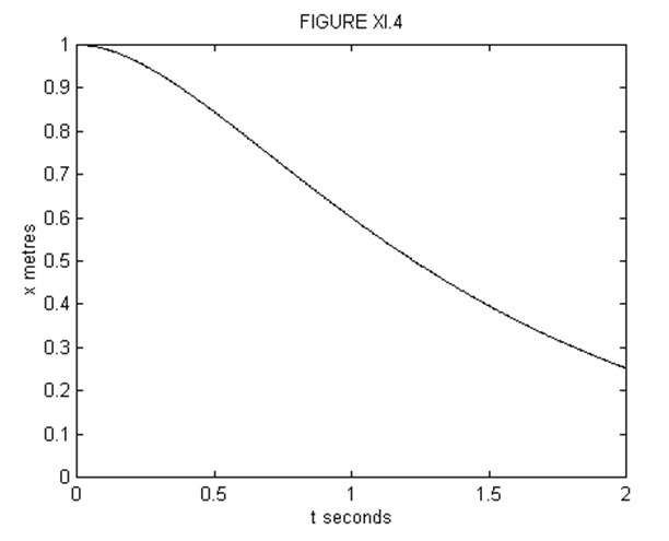
Figure XI.4 shows \( x\quad:\quad t\) for \(x_{0}\) = 1 m, \( \lambda_{1}\) = 1 s-1, \( \lambda_{2}\) = 2 s-1.
The displacement will fall to half of its initial value at a time given by putting \( \frac{x}{x_{0}}=\frac{1}{2}\) in Equation \( \ref{11.5.25}\). This will in general require a numerical solution. In our example, however, the equation reduces to \( \frac{1}{2}=2e^{-t}-e^{-2t}\) and if we let \( u=e^{-t}\), this becomes \( u^{2}-2u+\frac{1}{2}=0\). The two solutions of this are \( u=1.707107\) or \( 0.292893\). The first of these gives a negative t, so we want the second solution, which corresponds to \( t= 1.228\) seconds.
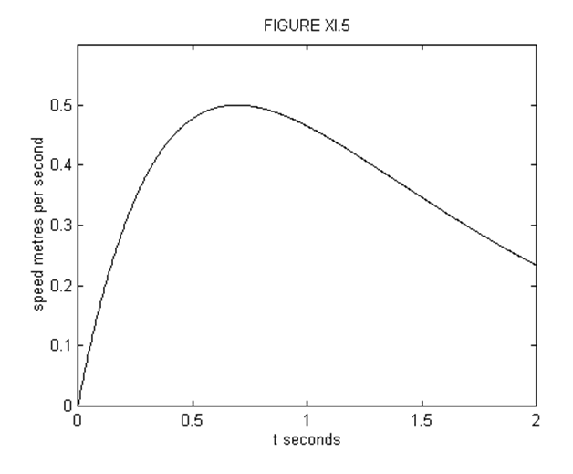
The velocity as a function of time is given by
\[ \dot{x}=-\frac{\lambda_{1}\lambda_{2}x_{0}}{\lambda_{2}-\lambda_{1}}(e^{-\lambda_{1}t}-e^{\lambda_{2}t}). \label{11.5.26a}\tag{11.5.26a} \]
This is always negative. In figure XI.5, is shown the speed, which is \( |\dot{x}|\) as a function of time, for our numerical example. Those who enjoy differentiating can show that the maximum speed is reached in a time \( -\dot{x}\) and that the maximum speed is \( \frac{\lambda_{1}\lambda_{2}x_{0}}{\lambda_{2}-\lambda_{1}}[(\frac{\lambda_{1}}{\lambda_{2}})^{\frac{\lambda_{2}}{\lambda_{2}-\lambda_{1}}}-(\frac{\lambda_{1}}{\lambda_{2}})^{\frac{\lambda_{1}}{\lambda_{2}-\lambda_{1}}}]\). (Are these dimensionally correct?) In our example, the maximum speed, reached at \( t=\ln 2=0.6931\) seconds, is 0.5 m s-1.
\( x_{0}=0,\quad (\dot{x})_{0}=V(>0)\).
In this case it is easy to show that
\[ x=\frac{V}{\lambda_{2}-\lambda_{1}}(e^{-\lambda_{1}t}-e^{-\lambda_{2}t}). \label{11.5.26b}\tag{11.5.26b} \]
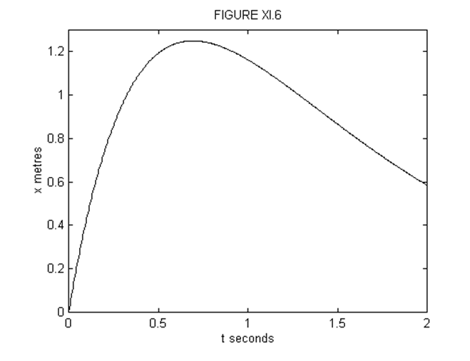
It is left as an exercise to show that \( x\) reaches a maximum value of \( \frac{V}{\lambda_{2}}(\frac{\lambda_{1}}{\lambda_{2}})^{\frac{\lambda_{1}}{\lambda_{2}-\lambda_{1}}}\) when \( t=\frac{\ln(\frac{\lambda_{2}}{\lambda_{1}})}{\lambda_{2}-\lambda_{1}}\). Figure XI.6 illustrates Equation \( \ref{11.5.26a}\) for \( \lambda_{1}\) = 1 s-1, \( \lambda_{2}\) = 2 s-1, \( V\) = 5 m s-1. The maximum displacement of 1.25 m is reached when \( t = \ln 2 = 0.6831\) s. It is also left as an exercise to show that equation \( \ref{11.5.26a}\) can be written
\[ x=\frac{2Ve^{-\frac{1}{2}\lambda t}}{\lambda_{2}-\lambda_{1}}\sinh (\frac{1}{4}\gamma^{2}-\omega_{0}^{2}). \label{11.5.27}\tag{11.5.27} \]
\( x_{0}\neq 0,\quad(\dot{x})_{0}=-V\).
This is the really exciting example, because the suspense-filled question is whether the particle will shoot past the origin at some finite time and then fall back to the origin; or whether it will merely tamely fall down asymptotically to the origin without ever crossing it. The tension will be almost unbearable as we find out. In fact, I cannot wait; I am going to plot \( x\) versus \( t\) in figure XI.7 for \( \lambda_{1}\) = 1 s-1, \( \lambda_{2}\) = 2 s -1, \( x_{0}\) = 1 m, and three different values of \( V\), namely 1, 2 and 3 m s-1.
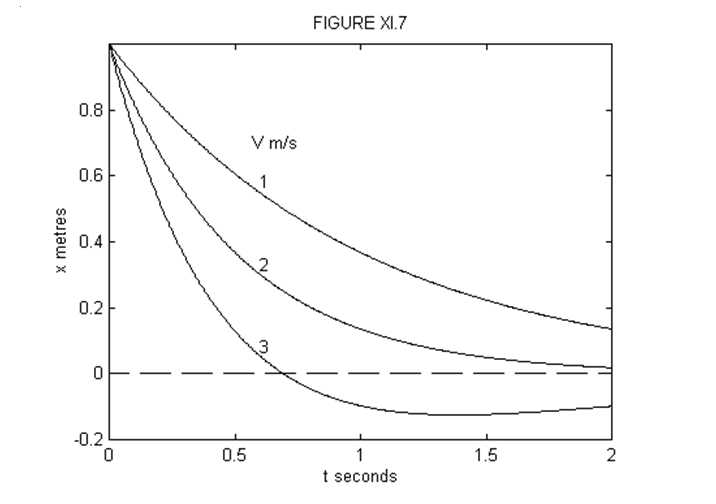
We see that if \( V\) = 3 m s-1 the particle overshoots the origin after about 0.7 seconds. If \( V\) = 1 m s-1, it does not look as though it will ever reach the origin. And if \( V\) = 2 m s-1, I'm not sure. Let's see what we can do. We can find out when it crosses the origin by putting \( x\)= 0 in Equation \( \ref{11.5.20}\), where \( A\) and \( B\) are found from Equations \( \ref{11.5.24}\) with \( (\dot{x})_{0}=-V\). This gives, for the time when it crosses the origin,
\[ t=\frac{1}{\lambda_{2}-\lambda_{1}}\ln(\frac{V-\lambda_{1}x_{0}}{V-\lambda_{2}x_{0}}). \label{11.5.28}\tag{11.5.28} \]
Since \( \lambda_{2} > \lambda_{1}\), this implies that the particle will overshoot the origin if \( V > \lambda_{2}x_{0}\), and this in turn implies that, for a given \( V\), it will overshoot only if
\[ \gamma < \frac{\frac{V^{2}}{x_{0}^{2}}+\omega_{0}^{2}}{\frac{V}{x_{0}}}. \label{11.5.29}\tag{11.5.29} \]
For our example, \( \lambda_{2}x_{0}\)= 2 m s-1, so that it just fails to overshoot the origin if \( V\)= 2 m s-1. For \( V\) = 3 m s-1, it crosses the origin at \(t=\ln 2=0.6931\) s. In order to find out how far past the origin it goes, and when, we can do this just as in
I make it that it reaches its maximum negative displacement of -0.125 m at \( t = \ln 4 = 1.386\) s.