14.6: Spring Force Energy Diagram

The spring force on an object is a restoring force \(\overrightarrow{\mathbf{F}}^{s}=F_{x}^{s} \hat{\mathbf{i}}=-k x \hat{\mathbf{i}}\) where we choose a coordinate system with the equilibrium position at \(x_{i}=0\) and x is the amount the spring has been stretched \((x>0)\) or compressed \((x<0)\) from its equilibrium position. We calculate the potential energy difference Equation (14.4.9) and found that

\[U^{s}(x)-U^{s}\left(x_{i}\right)=-\int_{x_{i}}^{x} F_{x}^{s} d x=\frac{1}{2} k\left(x^{2}-x_{i}^{2}\right) \nonumber \]

The first fundamental theorem of calculus states that

\[U(x)-U\left(x_{i}\right)=\int_{x^{\prime}=x_{i}} x^{x^{\prime}=x} \frac{d U}{d x^{\prime}} d x^{\prime} \nonumber \]

Comparing Equation (14.5.1) with Equation (14.5.2) shows that the force is the negative derivative (with respect to position) of the potential energy,

\[F_{x}^{s}=-\frac{d U^{s}(x)}{d x} \nonumber \]

Choose the zero reference point for the potential energy to be at the equilibrium position, \(U^{s}(0) \equiv 0\) Then the potential energy function becomes

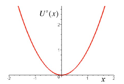
\(U^{s}(x)=\frac{1}{2} k x^{2}\)

\[F_{x}^{s}=-\frac{d U^{s}(x)}{d x}=-\frac{d}{d x}\left(\frac{1}{2} k x^{2}\right)=-k x \nonumber \]

In Figure 14.9 we plot the potential energy function \(U^{s}(x)\) for the spring force as function of x with \(U^{s}(0) \equiv 0\) (the units are arbitrary).

Figure 14.9 Graph of potential energy function as function of x for the spring.

The minimum of the potential energy function occurs at the point where the first derivative vanishes

\(\frac{d U^{s}(x)}{d x}=0\)

From Equation (14.5.4), the minimum occurs at x = 0,

\[0=\frac{d U^{s}(x)}{d x}=k x \nonumber \]

Because the force is the negative derivative of the potential energy, and this derivative vanishes at the minimum, we have that the spring force is zero at the minimum \(x=0\) agreeing with our force law, \(\left.F_{x}^{s}\right|_{x=0}=-\left.k x\right|_{x=0}=0\).

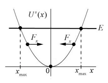
The potential energy function has positive curvature in the neighborhood of a minimum equilibrium point. If the object is extended a small distance \(x>0\) away from equilibrium, the slope of the potential energy function is positive, \(d U(x) / d x>0\), hence the component of the force is negative because \(F_{x}=-d U(x) / d x<0\). Thus the object experiences a restoring force towards the minimum point of the potential. If the object is compresses with \(x<0\) then \(d U(x) / d x<0\), hence the component of the force is positive, \(F_{x}=-d U(x) / d x>0\) and the object again experiences a restoring force back towards the minimum of the potential energy as in Figure 14.10.

Figure 14.10 Stability diagram for the spring force

The mechanical energy at any time is the sum of the kinetic energy K x( ) and the potential energy \(U^{s}(x)\)

\(E_{m}=K(x)+U^{s}(x)\)

Suppose our spring-object system has no loss of mechanical energy due to dissipative forces such as friction or air resistance. Both the kinetic energy and the potential energy are functions of the position of the object with respect to equilibrium. The energy is a constant of the motion and with our choice of \(U^{s}(0) \equiv 0\), the energy can be either a positive value or zero. When the energy is zero, the object is at rest at the equilibrium position.

In Figure 14.10, we draw a straight horizontal line corresponding to a non-zero positive value for the energy \(E_{m}\) on the graph of potential energy as a function of x . The energy intersects the potential energy function at two points \(\left\{-x_{\max }, x_{\max }\right\} \text { with } x_{\max }>0\). These points correspond to the maximum compression and maximum extension of the spring, which are called the turning points. The kinetic energy is the difference between the energy and the potential energy,

\[K(x)=E_{m}-U^{s}(x) \nonumber \]

At the turning points, where \(E_{m}=U^{s}(x)\), the kinetic energy is zero. Regions where the kinetic energy is negative, \(x<-x_{\max } \text { or } x>x_{\max }\) are called the classically forbidden regions, which the object can never reach if subject to the laws of classical mechanics. In quantum mechanics, with similar energy diagrams for quantum systems, there is a very small probability that the quantum object can be found in a classically forbidden region.

Example 14.1 Energy Diagram

The potential energy function for a particle of mass m , moving in the x -direction is given by

\[U(x)=-U_{1}\left(\left(\frac{x}{x_{1}}\right)^{3}-\left(\frac{x}{x_{1}}\right)^{2}\right) \nonumber \]

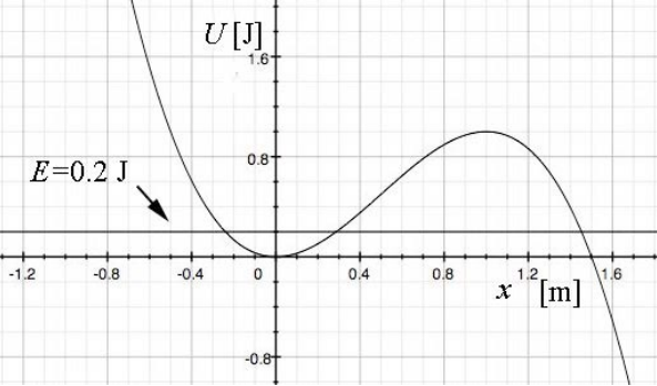
where \(U_{1}\) and \(x_{1}\) are positive constants and \(U(0)=0\). (a) Sketch \(U(x) / U_{1}\) as a function of \(x / x_{1}\). (b) Find the points where the force on the particle is zero. Classify them as stable or unstable. Calculate the value of \(U(x) / U_{1}\) at these equilibrium points. (c) For energies E that lies in \(0<E<(4 / 27) U_{1}\) find an equation whose solution yields the turning points along the x-axis about which the particle will undergo periodic motion. (d) Suppose \(E=(4 / 27) U_{1}\) and that the particle starts at \(x=0\) with speed \(v_{0}\). Find \(v_{0}\).

Solution: a) Figure 14.11 shows a graph of U(x) vs. x , with the choice of values \(x_{1}=1.5 \mathrm{m}\) \(U_{1}=27 / 4 \mathrm{J}, \text { and } E=0.2 \mathrm{J}\).

Figure 14.11 Energy diagram for Example 14.1

b) The force on the particle is zero at the minimum of the potential which occurs at

\[F_{x}(x)=-\frac{d U}{d x}(x)=U_{1}\left(\left(\frac{3}{x_{1}^{3}}\right) x^{2}-\left(\frac{2}{x_{1}^{2}}\right) x\right)=0 \nonumber \]

which becomes

\[x^{2}=\left(2 x_{1} / 3\right) x \nonumber \]

We can solve Equation (14.5.12) for the extrema. This has two solutions

\(x=\left(2 x_{1} / 3\right)\) and \(\\begin{equation}x=0\end{equation})

The second derivative is given by

\[\frac{d^{2} U}{d x^{2}}(x)=-U_{1}\left(\left(\frac{6}{x_{1}^{3}}\right) x-\left(\frac{2}{x_{1}^{2}}\right)\right) \nonumber \]

Evaluating the second derivative at \(x=\left(2 x_{1} / 3\right)\) yields a negative quantity

\[\frac{d^{2} U}{d x^{2}}\left(x=\left(2 x_{1} / 3\right)\right)=-U_{1}\left(\left(\frac{6}{x_{1}^{3}}\right) \frac{2 x_{1}}{3}-\left(\frac{2}{x_{1}^{2}}\right)\right)=-\frac{2 U_{1}}{x_{1}^{2}}<0 \nonumber \]

indicating the solution \(x=\left(2 x_{1} / 3\right)\) represents a local maximum and hence is an unstable point. At \(x=\left(2 x_{1} / 3\right)\), , the potential energy is given by the value \(U\left(\left(2 x_{1} / 3\right)\right)=(4 / 27) U_{1}\). Evaluating the second derivative at x = 0 yields a positive quantity

\[\frac{d^{2} U}{d x^{2}}(x=0)=-U_{1}\left(\left(\frac{6}{x_{1}^{3}}\right) 0-\left(\frac{2}{x_{1}^{2}}\right)\right)=\frac{2 U_{1}}{x_{1}^{2}}>0 \nonumber \]

indicating the solution x=0 represents a local minimum and is a stable point. At the local minimum x = 0, the potential energy U(0) = 0.

c) Consider a fixed value of the energy of the particle within the range

\[U(0)=0<E<U\left(2 x_{1} / 3\right)=\frac{4 U_{1}}{27} \nonumber \]

If the particle at any time is found in the region \(x_{a}<x<x_{b}<2 x_{1} / 3\), where \(x_{a}\) and \(x_{b}\) are the turning points and are solutions to the equation

\[E=U(x)=-U_{1}\left(\left(\frac{x}{x_{1}}\right)^{3}-\left(\frac{x}{x_{1}}\right)^{2}\right) \nonumber \]

then the particle will undergo periodic motion between the values \(x_{a}<x<x_{b}\). Within this region \(x_{a}<x<x_{b}\), the kinetic energy is always positive because \(K(x)=E-U(x)\) There is another solution \(x_{c}\) to Equation (14.5.18) somewhere in the region \(x_{c}>2 x_{1} / 3\). If the particle at any time is in the region \(x>x_{c}\) then it at any later time it is restricted to the region \(x_{c}<x<+\infty\).

For \(E>U\left(2 x_{1} / 3\right)=(4 / 27) U_{1}\), , Equation (14.5.18) has only one solution \(x_{d}\). . For all values of \(x>x_{d}\), the kinetic energy is positive, which means that the particle can “escape” to infinity but can never enter the region \(x<x_{d}\).

For \(E<U(0)=0\) the kinetic energy is negative for the range \(-\infty<x<x_{e}\) where \(x_{e}\) satisfies Equation (14.5.18) and therefore this region of space is forbidden.

(d) If the particle has speed \(v_{0}\) at x = 0 where the potential energy is zero, \(U(0)=0\), the energy of the particle is constant and equal to kinetic energy

\[E=K(0)=\frac{1}{2} m v_{0}^{2} \nonumber \]

Therefore

\[(4 / 27) U_{1}=\frac{1}{2} m v_{0}^{2} \nonumber \]

which we can solve for the speed

\[v_{0}=\sqrt{8 U_{1} / 27 m} \nonumber \]