3.5: Elastic Scattering

If \(E>0\), the motion is unbound for any realistic interaction potential. In this case, the two most important parameters of the particle trajectory are the impact parameter \(b\) and the scattering angle \(\theta\) (Figure 9), and the main task for theory is to find the relation between them in the given potential \(U(r)\).

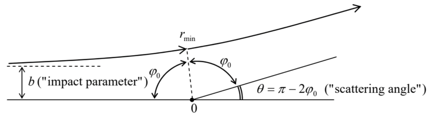Figure 3.9. Main geometric parameters of the scattering problem.

For that, it is convenient to note that \(b\) is related to the two conserved quantities, particle’s energy \(^{22} E\) and its angular momentum \(L_{z}\), in a simple way. Indeed, at \(r \gg b\), the definition \(\mathbf{L}=\mathbf{r} \times(m \mathbf{v})\) yields \(L_{z}=b m v_{\infty}\), where \(v_{\infty}=(2 E / m)^{1 / 2}\) is the initial (and hence the final) velocity of the particle, so that \[L_{z}=b(2 m E)^{1 / 2} .\] Hence the angular contribution to the effective potential (44) may be represented as \[\frac{L_{z}^{2}}{2 m r^{2}}=E \frac{b^{2}}{r^{2}} .\] Second, according to Eq. (48), the trajectory sections going from infinity to the nearest approach point \(\left(r=r_{\min }\right)\) and from that point to infinity, have to be similar, and hence correspond to equal angle changes \(\varphi_{0}-\) see Figure 9. Hence we may apply the general Eq. (48) to just one of the sections, say \(\left[r_{\min }\right.\), \(\infty\) ], to find the scattering angle: \[\theta=\pi-2 \varphi_{0}=\pi-2 \frac{L_{z}}{(2 m)^{1 / 2}} \int_{r_{\min }}^{\infty} \frac{d r}{r^{2}\left[E-U(r)-L_{z}^{2} / 2 m r^{2}\right]^{1 / 2}}=\pi-2 \int_{r_{\min }}^{\infty} \frac{b d r}{r^{2}\left[1-U(r) / E-b^{2} / r^{2}\right]^{1 / 2}} .\] In particular, for the Coulomb potential (49), now with an arbitrary sign of \(\alpha\), we can apply the same table integral as in the previous section to get \({ }^{23}\) \[|\theta|=\left|\pi-2 \cos ^{-1} \frac{\alpha / 2 E b}{\left[1+(\alpha / 2 E b)^{2}\right]^{1 / 2}}\right| .\] This result may be more conveniently rewritten as \[\tan \frac{|\theta|}{2}=\frac{|\alpha|}{2 E b} \text {. }\] Very clearly, the scattering angle’s magnitude increases with the potential strength \(\alpha\), and decreases as either the particle energy or the impact parameter (or both) are increased.

The general result (68) and the Coulomb-specific relations (69) represent a formally complete solution of the scattering problem. However, in a typical experiment on elementary particle scattering, the impact parameter \(b\) of a single particle is unknown. In this case, our results may be used to obtain the statistics of the scattering angle \(\theta\), in particular, the so-called differential cross-section \(^{24}\) \[\frac{d \sigma}{d \Omega} \equiv \frac{1}{n} \frac{d N}{d \Omega},\] where \(n\) is the average number of the incident particles per unit area, and \(d N\) is the average number of the particles scattered into a small solid angle range \(d \Omega\). For a uniform beam of initial particles, \(d \sigma / d \Omega\) may be calculated by counting the average number of incident particles that have the impact parameters within a small range \(d b\) : \[d N=n 2 \pi b d b .\] and are scattered by a spherically-symmetric center, which provides an axially-symmetric scattering pattern, into the corresponding small solid angle range \(d \Omega=2 \pi|\sin \theta d \theta|\). Plugging these two equalities into Eq. \((70)\), we get the following general geometric relation: \[\frac{d \sigma}{d \Omega}=b\left|\frac{d b}{\sin \theta d \theta}\right| .\] In particular, for the Coulomb potential (49), a straightforward differentiation of Eq. (69) yields the so-called Rutherford scattering formula (reportedly derived by Ralph Howard Fowler): \[\frac{d \sigma}{d \Omega}=\left(\frac{\alpha}{4 E}\right)^{2} \frac{1}{\sin ^{4}(\theta / 2)}\] This result, which shows a very strong scattering to small angles (so strong that the integral that expresses the total cross-section \[\sigma \equiv \oint_{4 \pi} \frac{d \sigma}{d \Omega} d \Omega\] is diverging at \(\theta \rightarrow 0),{ }^{25}\) and very weak backscattering (to angles \(\theta \approx \pi\) ) was historically extremely significant: in the early 1910s: its good agreement with \(\alpha\)-particle scattering experiments carried out by Ernest Rutherford’s group gave a strong justification for his introduction of the planetary model of atoms, with electrons moving around very small nuclei - just as planets move around stars.

Note that elementary particle scattering is frequently accompanied by electromagnetic radiation and/or other processes leading to the loss of the initial mechanical energy of the system. Such inelastic scattering may give significantly different results. (In particular, capture of an incoming particle becomes possible even for a Coulomb attracting center.) Also, quantum-mechanical effects may be important at the scattering of light particles with relatively low energies, \({ }^{26}\) so that the above results should be used with caution.

---

\({ }^{22}\) The energy conservation law is frequently emphasized by calling such process elastic scattering.

\({ }^{23}\) Alternatively, this result may be recovered directly from the first form of Eq. (65), with the eccentricity \(e\) expressed via the same dimensionless parameter \((2 E b / \alpha): e=\left[1+(2 E b / \alpha)^{2}\right]^{1 / 2}>1\).

\({ }_{24}\) This terminology stems from the fact that an integral (74) of \(d \sigma / d \Omega\) over the full solid angle, called the total cross-section \(\sigma\), has the dimension of the area: \(\sigma=N / n\), where \(N\) is the total number of scattered particles.

\({ }^{25}\) This divergence, which persists at the quantum-mechanical treatment of the problem (see, e.g., QM Chapter 3), is due to particles with very large values of \(b\), and disappears at an account, for example, of any non-zero concentration of the scattering centers.

\({ }^{26}\) Their discussion may be found in QM Secs. \(3.3\) and 3.8.