3.6: Exercise Problems

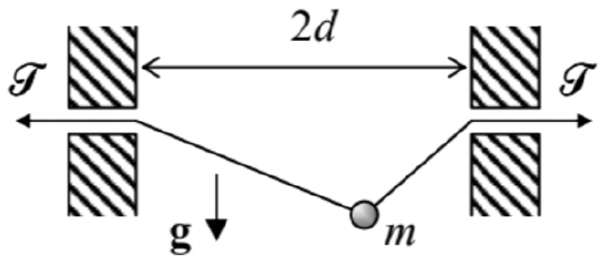
3.1. For the system considered in Problem \(2.6\) (a bead sliding along a string with fixed tension \(\mathscr{F}\), see the figure on the right), analyze small oscillations of the bead near the equilibrium.

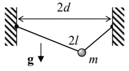
3.2. For the system considered in Problem \(2.7\) (a bead sliding along a string of a fixed length \(2 l\), see the figure on the right), analyze small oscillations near the equilibrium.

3.3. For a 1D particle of mass \(m\), placed into potential \(U(q)=\alpha q^{2 n}\) (where \(\alpha>0\), and \(n\) is a positive integer), calculate the functional dependence of the particle oscillation period \(\tau\) on its energy \(E\). Explore the limit \(n \rightarrow \infty\).

3.4. Explain why the term \(m r^{2} \dot{\varphi}^{2} / 2\), recast in accordance with Eq. (42), cannot be merged with \(U(r)\) in Eq. (38), to form an effective 1D potential energy \(U(r)-L_{z}^{2} / 2 m r^{2}\), with the second term’s sign opposite to that given by Eq. (44). We have done an apparently similar thing for our testbed, bead-onrotating-ring problem at the very end of Sec. 1 - see Eq. (6); why cannot the same trick work for the planetary problem? Besides a formal explanation, discuss the physics behind this difference.

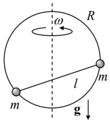
3.5. A system consisting of two equal masses \(m\) on a light rod of length \(l\) (frequently called a dumbbell) can slide without friction along a vertical ring of radius \(R\), rotated about its vertical diameter with constant angular velocity \(\omega-\) see the figure on the right. Derive the condition of stability of the lower horizontal position of the dumbbell.

3.6. Analyze the dynamics of the so-called spherical pendulum - a point mass hung, in a uniform gravity field \(\mathbf{g}\), on a light cord of length \(l\), with no motion’s confinement to a vertical plane. In particular:

(i) find the integrals of motion and reduce the problem to a \(1 \mathrm{D}\) one,

(ii) calculate the time period of the possible circular motion around the vertical axis, and

(iii) explore small deviations from the circular motion. (Are the pendulum orbits closed?) \({ }^{27}\)

3.7. The orbits of Mars and Earth around the Sun may be well approximated as circles, with a radii ratio of \(3 / 2\). Use this fact, and the Earth’s year duration (which you should know :-), to calculate the time of travel to Mars spending the least energy for spacecraft’s launch. Neglect the planets’ size and the effects of their gravitational fields.

3.8. Derive first-order and second-order differential equations for the reciprocal distance \(u \equiv 1 / r\) as a function of \(\varphi\), describing the trajectory of particle’s motion in a central potential \(U(r)\). Spell out the latter equation for the particular case of the Coulomb potential (49) and discuss the result.

3.9. For the motion of a particle in the Coulomb attractive field (with potential \(U(r)=-\alpha / r\), with \(\alpha>0\) ), calculate and sketch the so-called hodograph \(^{28}-\) the trajectory followed by the head of the velocity vector \(\mathbf{v}\), provided that its tail is kept at the origin.

3.10. For motion in the following central potential: \[U(r)=-\frac{\alpha}{r}+\frac{\beta}{r^{2}},\] (i) find the orbit \(r(\varphi)\), for positive \(\alpha\) and \(\beta\), and all possible ranges of energy \(E\);

(ii) prove that in the limit \(\beta \rightarrow 0\), and for energy \(E<0\), the orbit may be represented as a slowly rotating ellipse;

(iii) express the angular velocity of this slow orbit rotation via the parameters \(\alpha\) and \(\beta\), the particle’s mass \(m\), its energy \(E\), and the angular momentum \(L_{z}\).

3.11. A particle is moving in the field of an attractive central force, with potential \[U(r)=-\frac{\alpha}{r^{n}}, \quad \text { where } \alpha n>0 .\] For what values of \(n\) is a circular orbit stable?

3.12. Determine the condition for a particle of mass \(m\), moving under the effect of a central attractive force \[\mathbf{F}=-\alpha \frac{\mathbf{r}}{r^{3}} \exp \left\{-\frac{r}{R}\right\},\] where \(\alpha\) and \(R\) are positive constants, to have a stable circular orbit.

3.13. A particle of mass \(m\), with angular momentum \(L_{z}\), moves in the field of an attractive central force with a distance-independent magnitude \(F\). If particle’s energy \(E\) is slightly higher than the value \(E_{\min }\) corresponding to the circular orbit of the particle, what is the time period of its radial oscillations? Compare the period with that of the circular orbit at \(E=E_{\min }\).

3.14. For particle scattering by a repulsive Coulomb field, calculate the minimum approach distance \(r_{\min }\) and the velocity \(v_{\min }\) at that point, and analyze their dependence on the impact parameter \(b\) (see Figure 9) and the initial velocity \(v_{\infty}\) of the particle.

3.15. A particle is launched from afar, with impact parameter \(b\), toward an attracting center with \[U(r)=-\frac{\alpha}{r^{n}}, \quad \text { with } n>2, \alpha>0 .\] (i) Express the minimum distance between the particle and the center via \(b\), if the initial kinetic energy \(E\) of the particle is barely sufficient for escaping its capture by the attracting center.

(ii) Calculate the capture’s total cross-section; explore the limit \(n \rightarrow 2\).

3.16. A meteorite with initial velocity \(v_{\infty}\) approaches an atmosphere-free planet of mass \(M\) and radius \(R\).

(i) Find the condition on the impact parameter \(b\) for the meteorite to hit the planet’s surface.

(ii) If the meteorite barely avoids the collision, what is its scattering angle?

3.17. Calculate the differential and total cross-sections of the classical, elastic scattering of small particles by a hard sphere of radius \(R\).

3.18. The most famous \({ }^{29}\) confirmation of Einstein’s general relativity theory has come from the observation, by A. Eddington and his associates, of star light’s deflection by the Sun, during the May 1919 solar eclipse. Considering light photons as classical particles propagating with the speed of light, \(v_{0} \rightarrow c \approx 3.00 \times 10^{8} \mathrm{~m} / \mathrm{s}\), and the astronomic data for Sun’s mass, \(M_{\mathrm{S}} \approx 1.99 \times 10^{30} \mathrm{~kg}\), and radius, \(R_{\mathrm{S}} \approx\) \(6.96 \times 10^{8} \mathrm{~m}\), calculate the non-relativistic mechanics’ prediction for the angular deflection of the light rays grazing the Sun’s surface.

---

\({ }^{27}\) Solving this problem is a very good preparation for the analysis of symmetric top’s rotation in the next chapter.

\({ }^{28}\) The use of this notion for the characterization of motion may be traced back at least to an 1846 treatise by W. Hamilton. Nowadays, it is most often used in applied fluid mechanics, in particular meteorology.

\({ }^{29}\) It was not the first confirmation, though. The first one came four years earlier from Albert Einstein himself, who showed that his theory may qualitatively explain the difference between the rate of Mercury orbit’s precession, known from earlier observations, and the non-relativistic theory of that effect.