4.1: Translation and Rotation

It is natural to start a discussion of many-particle systems from a (relatively :-) simple limit when the changes of distances \(r_{k k^{\prime}} \equiv\left|\mathbf{r}_{\mathrm{k}}-\mathbf{r}_{\mathrm{k}^{\prime}}\right|\) between the particles are negligibly small. Such an abstraction is called the (absolutely) rigid body, and is a reasonable approximation in many practical problems, including the motion of solids. In other words, this model neglect deformations - which will be the subject of the next chapters. The rigid-body approximation reduces the number of degrees of freedom of the system of \(N\) particles from \(3 N\) to just six - for example, three Cartesian coordinates of one point (say, 0 ), and three angles of the system’s rotation about three mutually perpendicular axes passing through this point - see Figure \(1 .{ }^{1}\)

Figure 4.1. Deriving Eq. (8).

As it follows from the discussion in Secs. 1.1-3, any purely translational motion of a rigid body, at which the velocity vectors \(\mathbf{v}\) of all points are equal, is not more complex than that of a point particle. Indeed, according to Eqs. (1.8) and (1.30), in an inertial reference frame such a body moves, upon the effect of the net external force \(\mathbf{F}^{(\mathrm{ext})}\), exactly as a point particle. However, the rotation is a bit more tricky.

Let us start by showing that an arbitrary elementary displacement of a rigid body may be always considered as a sum of the translational motion discussed above, and what is called a pure rotation. For that, consider a "moving" reference frame, firmly bound to the body, and an arbitrary vector A (Figure 1). The vector may be represented by its Cartesian components \(A_{j}\) in that moving frame: \[\mathbf{A}=\sum_{j=1}^{3} A_{j} \mathbf{n}_{j} .\] Let us calculate the time derivative of this vector as observed from a different ("lab") frame, taking into account that if the body rotates relative to this frame, the directions of the unit vectors \(\mathbf{n}_{j}\), as seen from the lab frame, change in time. Hence, we have to differentiate both operands in each product contributing to the sum (1): \[\left.\frac{d \mathbf{A}}{d t}\right|_{\text {in lab }}=\sum_{j=1}^{3} \frac{d A_{j}}{d t} \mathbf{n}_{j}+\sum_{j=1}^{3} A_{j} \frac{d \mathbf{n}_{j}}{d t} .\] On the right-hand side of this equality, the first sum evidently describes the change of vector \(\mathbf{A}\) as observed from the moving frame. In the second sum, each of the infinitesimal vectors \(d \mathbf{n}_{j}\) may be represented by its Cartesian components: \[d \mathbf{n}_{j}=\sum_{j^{\prime}=1}^{3} d \varphi_{i j^{\prime}} \mathbf{n}_{j^{\prime}}\] where \(d \varphi_{i j^{\prime}}\) are some dimensionless scalar coefficients. To find out more about them, let us scalarmultiply each side of Eq. (3) by an arbitrary unit vector \(\mathbf{n}_{j "}\), and take into account the evident orthonormality condition: \[\mathbf{n}_{j^{\prime}} \cdot \mathbf{n}_{j^{\prime \prime}}=\delta_{j j^{\prime \prime}},\] where \(\delta_{j j \prime}\) is the Kronecker delta symbol. \({ }^{2}\) As a result, we get \[d \mathbf{n}_{j} \cdot \mathbf{n}_{j^{\prime \prime}}=d \varphi_{i j^{\prime \prime}}\] Now let us use Eq. (5) to calculate the first differential of Eq. (4): \[d \mathbf{n}_{j^{\prime}} \cdot \mathbf{n}_{j^{\prime \prime}}+\mathbf{n}_{j^{\prime}} \cdot d \mathbf{n}_{j^{\prime \prime}} \equiv d \varphi_{j j^{\prime \prime}}+d \varphi_{j^{\prime \prime \prime}}=0 ; \quad \text { in particular, } 2 d \mathbf{n}_{j} \cdot \mathbf{n}_{j}=2 d \varphi_{i j}=0 .\] These relations, valid for any choice of indices \(j, j\) ’, and \(j\) " of the set \(\{1,2,3\}\), show that the matrix of \(d \varphi_{i j}\) ’ is antisymmetric with respect to the swap of its indices; this means that there are not nine just three non-zero independent coefficients \(d \varphi_{i j}\), all with \(j \neq j\) ’. Hence it is natural to renumber them in a simpler way: \(d \varphi_{i j^{\prime}}=-d \varphi_{j^{\prime} j} \equiv d \varphi_{j "}\), where the indices \(j, j\) ’, and \(j\) " follow in the "correct" order - either \(\{1,2,3\}\), or \(\{2,3,1\}\), or \(\{3,1,2\}\). It is easy to check (either just by a component-by-component comparison or using the Levi-Civita permutation symbol \(\varepsilon_{i j j}{j}^{\prime, 3}\) ) that in this new notation, Eq. (3) may be represented just as a vector product: \[d \mathbf{n}_{j}=d \boldsymbol{\varphi} \times \mathbf{n}_{j},\] where \(d \varphi\) is the infinitesimal vector defined by its Cartesian components \(d \varphi_{j}\) in the rotating reference frame \(\left\{\mathbf{n}_{1}, \mathbf{n}_{2}, \mathbf{n}_{3}\right\}\) - see Eq. (3).

This relation is the basis of all rotation kinematics. Using it, Eq. (2) may be rewritten as \[\left.\frac{d \mathbf{A}}{d t}\right|_{\text {in lab }}=\left.\frac{d \mathbf{A}}{d t}\right|_{\text {in mov }}+\sum_{j=1}^{3} A_{j} \frac{d \boldsymbol{\varphi}}{d t} \times\left.\mathbf{n}_{j} \equiv \frac{d \mathbf{A}}{d t}\right|_{\text {in mov }}+\boldsymbol{\omega} \times \mathbf{A}, \quad \text { where } \boldsymbol{\omega} \equiv \frac{d \boldsymbol{\varphi}}{d t} .\] To reveal the physical sense of the vector \(\omega\), let us apply Eq. (8) to the particular case when \(\mathbf{A}\) is the radius vector \(\mathbf{r}\) of a point of the body, and the lab frame is selected in a special way: its origin has the same position and moves with the same velocity as that of the moving frame in the particular instant under consideration. In this case, the first term on the right-hand side of Eq. (8) is zero, and we get \[\left.\frac{d \mathbf{r}}{d t}\right|_{\text {in special lab frame }}=\boldsymbol{\omega} \times \mathbf{r},\] were vector \(\mathbf{r}\) itself is the same in both frames. According to the vector product definition, the particle velocity described by this formula has a direction perpendicular to the vectors \(\omega\) and \(\mathbf{r}\) (Figure 2), and magnitude \(\omega r \sin \theta\). As Figure 2 shows, the last expression may be rewritten as \(\omega \rho\), where \(\rho=r \sin \theta\) is the distance from the line that is parallel to the vector \(\omega\) and passes through the point 0 . This is of course just the pure rotation about that line (called the instantaneous axis of rotation), with the angular velocity \(\omega\). Since according to Eqs. (3) and (8), the angular velocity vector \(\omega\) is defined by the time evolution of the moving frame alone, it is the same for all points \(\mathbf{r}\), i.e. for the rigid body as a whole. Note that nothing in our calculations forbids not only the magnitude but also the direction of the vector \(\omega\), and thus of the instantaneous axis of rotation, to change in time (and in many cases it does); hence the name.

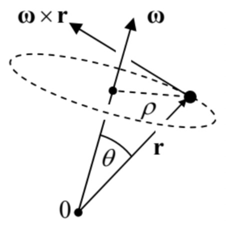Figure 4.2. The instantaneous axis and the angular velocity of rotation.

Now let us generalize our result a step further, considering two reference frames that do not rotate versus each other: one ("lab") frame arbitrary, and another one selected in the special way described above, so that for it Eq. (9) is valid in it. Since their relative motion of these two reference frames is purely translational, we can use the simple velocity addition rule given by Eq. (1.6) to write \[\left.\mathbf{v}\right|_{\text {in lab }}=\left.\mathbf{v}_{0}\right|_{\text {in lab }}+\left.\mathbf{v}\right|_{\text {in special lab frame }}=\left.\mathbf{v}_{0}\right|_{\text {in lab }}+\boldsymbol{\omega} \times \mathbf{r},\] where \(\mathbf{r}\) is the radius vector of a point is measured in the body-bound ("moving") frame 0.

---

\({ }^{1}\) An alternative way to arrive at the same number six is to consider three points of the body, which uniquely define its position. If movable independently, the points would have nine degrees of freedom, but since three distances \(r_{k k}\), between them are now fixed, the resulting three constraints reduce the number of degrees of freedom to six.

\({ }^{2}\) See, e.g., MA Eq. (13.1).

\({ }^{3}\) See, e,g., MA Eq. (13.2). Using this symbol, we may write \(d \varphi_{i j^{\prime}}=-d \varphi_{j j} \equiv \varepsilon_{j j j} d \varphi_{j^{\prime \prime}}\) for any choice of \(j, j^{\prime}\), and \(j\) ".