4.6: Non-inertial Reference Frames

To complete this chapter, let us use the results of our analysis of the rotation kinematics in Sec. 1 to complete the discussion of the transfer between two reference frames, started in the introductory Chapter 1. As Figure 12 (which reproduces Figure \(1.2\) in a more convenient notation) shows, even if the "moving" frame 0 rotates relative to the "lab" frame 0 ’, the radius vectors observed from these two frames are still related, at any moment of time, by the simple Eq. (1.5). In our new notation: \[\mathbf{r}^{\prime}=\mathbf{r}_{0}+\mathbf{r} \text {. }\]
between two reference frames.

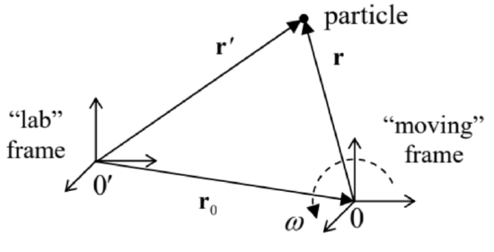Figure 4.12. The general case of transfer

However, as was mentioned in Sec. 1, for velocities the general addition rule is already more complex. To find it, let us differentiate Eq. (86) over time: \[\frac{d}{d t} \mathbf{r}^{\prime}=\frac{d}{d t} \mathbf{r}_{0}+\frac{d}{d t} \mathbf{r} .\] The left-hand side of this relation is evidently the particle’s velocity as measured in the lab frame, and the first term on the right-hand side is the velocity \(\mathbf{v}_{0}\) of the point 0 , as measured in the same lab frame. The last term is more complex: due to the possible mutual rotation of the frames 0 and 0 ’, that term may not vanish even if the particle does not move relative to the rotating frame 0 - see Figure 12 .

Fortunately, we have already derived the general Eq. (8) to analyze situations exactly like this one. Taking \(\mathbf{A}=\mathbf{r}\) in it, we may apply the result to the last term of Eq. (87), to get \[\left.\mathbf{v}\right|_{\text {in lab }}=\left.\mathbf{v}_{0}\right|_{\text {in lab }}+(\mathbf{v}+\boldsymbol{\omega} \times \mathbf{r}),\] where \(\omega\) is the instantaneous angular velocity of an imaginary rigid body connected to the moving reference frame (or we may say, of this frame as such), as measured in the lab frame 0’, while \(\mathbf{v}\) is \(d \mathbf{r} / d t\) as measured in the moving frame 0 . The relation (88), on one hand, is a natural generalization of Eq. (10) for \(\mathbf{v} \neq 0\); on the other hand, if \(\omega=0\), it is reduced to simple Eq. (1.8) for the translational motion of the frame 0 .

To calculate the particle’s acceleration, we may just repeat the same trick: differentiate Eq. (88) over time, and then use Eq. (8) again, now for the vector \(\mathbf{A}=\mathbf{v}+\omega \times \mathbf{r}\). The result is \[\left.\left.\mathbf{a}\right|_{\text {in lab }} \equiv \mathbf{a}_{0}\right|_{\text {in lab }}+\frac{d}{d t}(\mathbf{v}+\boldsymbol{\omega} \times \mathbf{r})+\boldsymbol{\omega} \times(\mathbf{v}+\boldsymbol{\omega} \times \mathbf{r}) .\] Carrying out the differentiation in the second term, we finally get the goal relation, \[\left.\left.\mathbf{a}\right|_{\text {in lab }} \equiv \mathbf{a}_{0}\right|_{\text {in lab }}+\mathbf{a}+\dot{\boldsymbol{\omega}} \times \mathbf{r}+2 \boldsymbol{\omega} \times \mathbf{v}+\boldsymbol{\omega} \times(\boldsymbol{\omega} \times \mathbf{r}),\] where \(\mathbf{a}\) is particle’s acceleration, as measured in the moving frame. This result is a natural generalization of the simple Eq. (1.9) to the rotating frame case.

Now let the lab frame 0 ’ be inertial; then the \(2^{\text {nd }}\) Newton law for a particle of mass \(m\) is \[\left.m \mathbf{a}\right|_{\text {in lab }}=\mathbf{F},\] where \(\mathbf{F}\) is the vector sum of all forces exerted on the particle. This is simple and clear; however, in many cases it is much more convenient to work in a non-inertial reference frame; for example, describing most phenomena on Earth’s surface, it is rather inconvenient to use a reference frame resting on the Sun (or in the galactic center, etc.). In order to understand what we should pay for the convenience of using a moving frame, we may combine Eqs. (90) and (91) to write \[m \mathbf{a}=\mathbf{F}-\left.m \mathbf{a}_{0}\right|_{\text {in lab }}-m \boldsymbol{\omega} \times(\boldsymbol{\omega} \times \mathbf{r})-2 m \boldsymbol{\omega} \times \mathbf{v}-m \dot{\boldsymbol{\omega}} \times \mathbf{r} .\] This result means that if we want to use a \(2^{\text {nd }}\) Newton law’s analog in a non-inertial reference frame, we have to add, to the actual net force \(\mathbf{F}\) exerted on a particle, four pseudo-force terms, called inertial forces, all proportional to particle’s mass. Let us analyze them one by one, always remembering that these are just mathematical terms, not actual forces. (In particular, it would be futile to seek for the \(3^{\text {rd }}\) Newton law’s counterpart for any inertial force.)

The first term, \(-\left.m \mathbf{a}_{0}\right|_{\text {in lab }}\), is the only one not related to rotation and is well known from the undergraduate mechanics. (Let me hope the reader remembers all these weight-in-the-moving-elevator problems.) However, despite its simplicity, this term has more subtle consequences. As an example, let us consider, semi-qualitatively, the motion of a planet, such as our Earth, orbiting a star and also rotating about its own axis - see Figure 13. The bulk-distributed gravity forces, acting on a planet from its star, are not quite uniform, because they obey the \(1 / r^{2}\) gravity law (1.15), and hence are equivalent to a single force applied to a point A slightly offset from the planet’s center of mass 0 , toward the star. For a spherically-symmetric planet, the direction from 0 to A would be exactly aligned with the direction toward the star. However, real planets are not absolutely rigid, so that, due to the centrifugal "force" (to be discussed imminently), the rotation about their own axis makes them slightly ellipsoidal - see Figure 13. (For our Earth, this equatorial bulge is about \(10 \mathrm{~km}\).) As a result, the net gravity force does create a small torque relative to the center of mass 0 . On the other hand, repeating all the arguments of this section for a body (rather than a point), we may see that, in the reference frame moving with the planet, the inertial force \(-M \mathbf{a}_{0}\) (with the magnitude of the total gravity force, but directed from the star) is applied exactly to the center of mass and hence does not create a torque about it. As a result, this pair of forces creates a torque \(\tau\) perpendicular to both the direction toward the star and the vector 0A. (In Figure 13 , the torque vector is perpendicular to the plane of the drawing). If the angle \(\delta\) between the planet’s "polar" axis of rotation and the direction towards the star was fixed, then, as we have seen in the previous section, this torque would induce a slow axis precession about that direction.

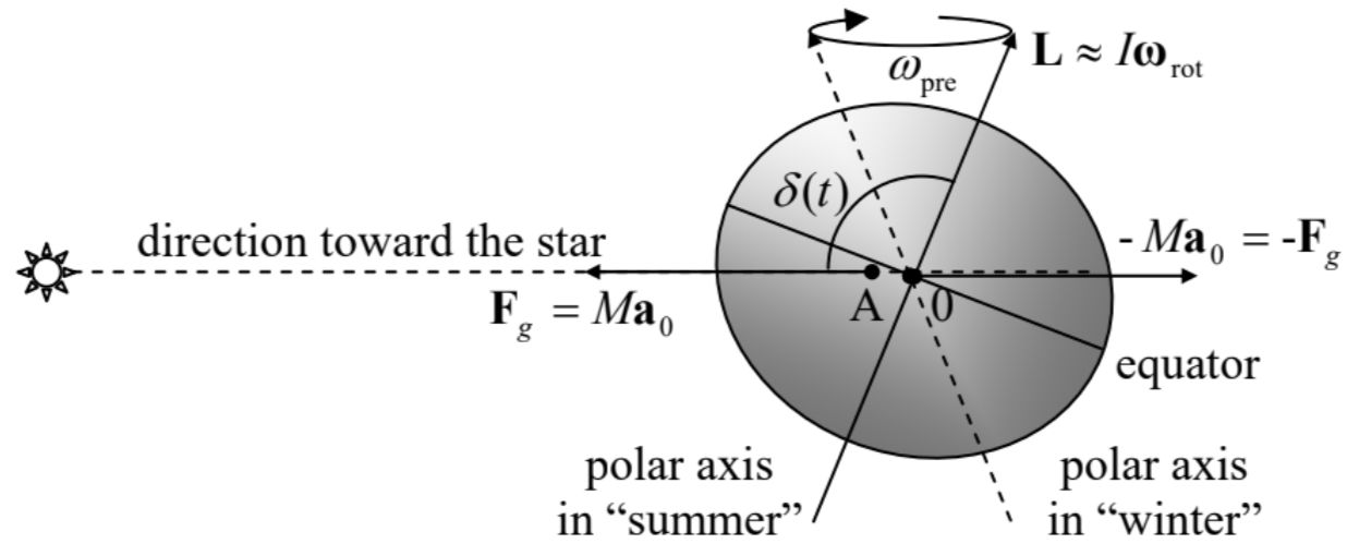Figure 4.13. The axial precession of a planet (with the equatorial bulge and the 0A-offset strongly exaggerated).

However, as a result of the orbital motion, the angle \(\delta\) oscillates in time much faster (once a year) between values \((\pi / 2+\varepsilon)\) and \((\pi / 2-\varepsilon)\), where \(\varepsilon\) is the axis tilt, i.e. angle between the polar axis (the direction of vectors \(\mathbf{L}\) and \(\omega_{\text {rot }}\) ) and the normal to the ecliptic plane of the planet’s orbit. (For the Earth, \(\varepsilon \approx 23.4^{\circ} .\) ) A straightforward averaging over these fast oscillations \(^{22}\) shows that the torque leads to the polar axis’ precession about the axis perpendicular to the ecliptic plane, keeping the angle \(\varepsilon\) constant \(-\) see Figure 13. For the Earth, the period \(T_{\text {pre }}=2 \pi / \omega_{\text {pre }}\) of this precession of the equinoxes, corrected to a substantial effect of Moon’s gravity, is close to 26,000 years. \({ }^{23}\)

Returning to Eq. (92), the direction of the second term of its right-hand side, \[\mathbf{F}_{\text {cf }} \equiv-m \boldsymbol{\omega} \times(\boldsymbol{\omega} \times \mathbf{r}),\] called the centrifugal force, is always perpendicular to, and directed out of the instantaneous rotation axis - see Figure 14. Indeed, the vector \(\omega \times \mathbf{r}\) is perpendicular to both \(\omega\) and \(\mathbf{r}\) (in Figure 14, normal to the drawing plane and directed from the reader) and has the magnitude \(\omega r \sin \theta=\omega \rho\), where \(\rho\) is the distance of the particle from the rotation axis. Hence the outer vector product, with the account of the minus sign, is normal to the rotation axis \(\omega\), directed from this axis, and is equal to \(\omega^{2} r \sin \theta=\omega^{2} \rho\). The "centrifugal force" is of course just the result of the fact that the centripetal acceleration \(\omega^{2} \rho\), explicit in the inertial reference frame, disappears in the rotating frame. For a typical location of the Earth \(\left(\rho \sim R_{\mathrm{E}} \approx 6 \times 10^{6} \mathrm{~m}\right)\), with its angular velocity \(\omega_{\mathrm{E}} \approx 10^{-4} \mathrm{~s}^{-1}\), the acceleration is rather considerable, of the order of \(3 \mathrm{~cm} / \mathrm{s}^{2}\), i.e. \(\sim 0.003 \mathrm{~g}\), and is responsible, in particular, for the largest part of the equatorial bulge mentioned above.

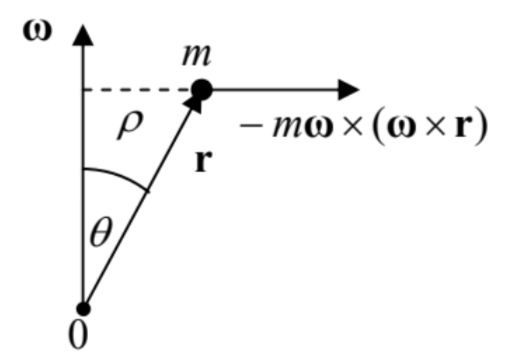Fig. 4.14. The centrifugal force.

As an example of using the centrifugal force concept, let us return again to our "testbed" problem on the bead sliding along a rotating ring - see Figure 2.1. In the non-inertial reference frame attached to the ring, we have to add, to the actual forces \(m \mathbf{g}\) and \(\mathbf{N}\) acting on the bead, the horizontal centrifugal force \({ }^{24}\) directed from the rotation axis, with the magnitude \(m \omega^{2} \rho\). Its component tangential to the ring equals \(\left(m \omega^{2} \rho\right) \cos \theta=m \omega^{2} R \sin \theta \cos \theta\), and hence the component of Eq. (92) along this direction is \(m a=-m g \sin \theta+m \omega^{2} R \sin \theta \cos \theta\). With \(a=R \ddot{\theta}\), this gives us an equation of motion equivalent to Eq. (2.25), which had been derived in Sec. \(2.2\) (in the inertial frame) using the Lagrangian formalism.

The third term on the right-hand side of Eq. (92), \[\mathbf{F}_{\mathrm{C}} \equiv-2 m \boldsymbol{\omega} \times \mathbf{v},\] is the so-called Coriolis force \({ }^{25}\) which is different from zero only if the particle moves in the rotating reference frame. Its physical sense may be understood by considering a projectile fired horizontally, say from the North Pole - see Figure 15.

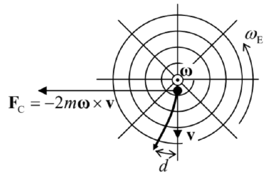Figure 4.15. The trajectory of a projectile fired horizontally from the North Pole, from the point of view of an Earth-bound observer looking down. The circles show parallels, while the straight lines mark meridians.

From the point of view of the Earth-based observer, the projectile will be affected by an additional Coriolis force (94), directed westward, with magnitude \(2 m \omega_{\mathrm{E}} v\), where \(\mathbf{v}\) is the main, southward component of the velocity. This force would cause the westward acceleration \(a=2 \omega_{\mathrm{E}} v\), and hence the westward deviation growing with time as \(d=a t^{2} / 2=\omega_{\mathrm{E}} v t^{2}\). (This formula is exact only if \(d\) is much smaller than the distance \(r=v t\) passed by the projectile.) On the other hand, from the point of view of an inertial-frame observer, the projectile’s trajectory in the horizontal plane is a straight line. However, during the flight time \(t\), the Earth surface slips eastward from under the trajectory by the distance \(d=r \varphi=(v t)\left(\omega_{\mathrm{E}} t\right)=\omega_{\mathrm{E}} v t^{2}\), where \(\varphi=\omega_{\mathrm{E}} t\) is the azimuthal angle of the Earth rotation during the flight). Thus, both approaches give the same result - as they should.

Hence, the Coriolis "force" is just a fancy (but frequently very convenient) way of description of a purely geometric effect pertinent to the rotation, from the point of view of the observer participating in it. This force is responsible, in particular, for the higher right banks of rivers in the Northern hemisphere, regardless of the direction of their flow - see Figure 16. Despite the smallness of the Coriolis force (for a typical velocity of the water in a river, \(v \sim 1 \mathrm{~m} / \mathrm{s}\), it is equivalent to acceleration \(a_{\mathrm{C}} \sim 10^{-2}\) \(\mathrm{cm} / \mathrm{s}^{2} \sim 10^{-5} \mathrm{~g}\) ), its multi-century effects may be rather prominent. \({ }^{26}\)

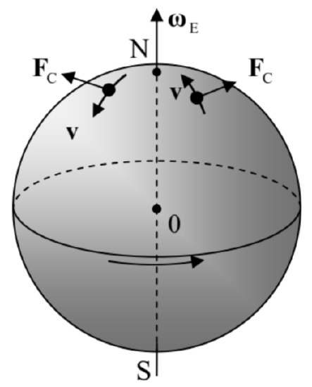Figure 4.16. Coriolis forces due to Earth’s rotation, in the Northern hemisphere.

Finally, the last, fourth term of Eq. (92), \(-m \dot{\boldsymbol{\omega}} \times \mathbf{r}\), exists only when the rotation frequency changes in time, and may be interpreted as a local-position-specific addition to the first term.The key relation (92), derived above from the Newton equation (91), may be alternatively obtained from the Lagrangian approach, which gives, as a by-product, some important insights on the momentum, as well as on the relation between \(E\) and \(H\), at rotation. Let us use Eq. (88) to represent the kinetic energy of the particle in an inertial "lab" frame in terms of \(\mathbf{v}\) and \(\mathbf{r}\) measured in a rotating frame: \[T=\frac{m}{2}\left[\left.\mathbf{v}_{0}\right|_{\text {in lab }}+(\mathbf{v}+\boldsymbol{\omega} \times \mathbf{r})\right]^{2},\] and use this expression to calculate the Lagrangian function. For the relatively simple case of a particle’s motion in the field of potential forces, measured from a reference frame that performs a pure rotation (so that \(\mathbf{v}_{0}\) |in lab \(=0\) ) \({ }^{27}\) with a constant angular velocity \(\omega\), we get \[L \equiv T-U=\frac{m}{2} v^{2}+m \mathbf{v} \cdot(\boldsymbol{\omega} \times \mathbf{r})+\frac{m}{2}(\boldsymbol{\omega} \times \mathbf{r})^{2}-U \equiv \frac{m}{2} v^{2}+m \mathbf{v} \cdot(\boldsymbol{\omega} \times \mathbf{r})-U_{\mathrm{ef}},\] where the effective potential energy,\({ }^{28}\) \[U_{\mathrm{ef}} \equiv U+U_{\mathrm{cf}}, \quad \text { with } U_{\mathrm{cf}} \equiv-\frac{m}{2}(\boldsymbol{\omega} \times \mathbf{r})^{2},\] is just the sum of the actual potential energy \(U\) of the particle and the so-called centrifugal potential energy, associated with the centrifugal force (93): \[\mathbf{F}_{\mathrm{cf}}=-\nabla U_{\mathrm{cf}}=-\nabla\left[-\frac{m}{2}(\boldsymbol{\omega} \times \mathbf{r})^{2}\right]=-m \boldsymbol{\omega} \times(\boldsymbol{\omega} \times \mathbf{r})\] It is straightforward to verify that the Lagrangian equations of motion derived from Eqs. (96), considering the Cartesian components of \(\mathbf{r}\) and \(\mathbf{v}\) as generalized coordinates and velocities, coincide with Eq. (92) (with \(\left.\mathbf{a}_{0}\right|_{\text {in lab }}=0, \dot{\boldsymbol{\omega}}=0\), and \(\mathbf{F}=-\nabla U\) ). Now it is very informative to have a look at a byproduct of this calculation, the generalized momentum (2.31) corresponding to the particle’s coordinate \(\mathbf{r}\) as measured in the rotating reference frame, \({ }^{29}\) \[\boldsymbol{h} \equiv \frac{\partial L}{\partial \mathbf{v}}=m(\mathbf{v}+\boldsymbol{\omega} \times \mathbf{r})\] According to Eq. (88) with \(\left.\mathbf{v}_{0}\right|_{\text {in lab }}=0\), the expression in the parentheses is just \(\left.\mathbf{v}\right|_{\text {in lab. However, from }}\) the point of view of the moving frame, i.e. not knowing about the simple physical sense of the vector \(\boldsymbol{p}\), we would have a reason to speak about two different linear momenta of the same particle, the so-called kinetic momentum \(\mathbf{p}=m \mathbf{v}\) and the canonical momentum \(\boldsymbol{\mu}=\mathbf{p}+m \omega \times \mathbf{r} .{ }^{30}\)

Now let us calculate the Hamiltonian function \(H\), defined by Eq. (2.32), and the energy \(E\) as functions of the same moving-frame variables: \[\begin{aligned} &H \equiv \sum_{j=1}^{3} \frac{\partial L}{\partial v_{j}} v_{j}-L=\boldsymbol{\mu} \cdot \mathbf{v}-L=m(\mathbf{v}+\boldsymbol{\omega} \times \mathbf{r}) \cdot \mathbf{v}-\left[\frac{m}{2} v^{2}+m \mathbf{v} \cdot(\boldsymbol{\omega} \times \mathbf{r})-U_{\mathrm{ef}}\right]=\frac{m v^{2}}{2}+U_{\mathrm{ef}}, \\ &E \equiv T+U=\frac{m}{2} v^{2}+m \mathbf{v} \cdot(\boldsymbol{\omega} \times \mathbf{r})+\frac{m}{2}(\boldsymbol{\omega} \times \mathbf{r})^{2}+U=\frac{m}{2} v^{2}+U_{\mathrm{ef}}+m \mathbf{v} \cdot(\boldsymbol{\omega} \times \mathbf{r})+m(\boldsymbol{\omega} \times \mathbf{r})^{2} . \end{aligned}\] These expressions clearly show that \(E\) and \(H\) are not equal. \({ }^{31}\) In hindsight, this is not surprising, because the kinetic energy (95), expressed in the moving-frame variables, includes a term linear in \(\mathbf{v}\), and hence is not a quadratic-homogeneous function of this generalized velocity. The difference of these functions may be represented as \[E-H=m \mathbf{v} \cdot(\boldsymbol{\omega} \times \mathbf{r})+m(\boldsymbol{\omega} \times \mathbf{r})^{2} \equiv m(\mathbf{v}+\boldsymbol{\omega} \times \mathbf{r}) \cdot(\boldsymbol{\omega} \times \mathbf{r})=\left.m \mathbf{v}\right|_{\text {in lab }} \cdot(\boldsymbol{\omega} \times \mathbf{r}) .\] Now using the operand rotation rule again, we may transform this expression into a simpler form: \({ }^{32}\) \[E-H=\boldsymbol{\omega} \cdot\left(\mathbf{r} \times\left. m \mathbf{v}\right|_{\text {in lab }}\right)=\boldsymbol{\omega} \cdot(\mathbf{r} \times \boldsymbol{\mu})=\left.\boldsymbol{\omega} \cdot \mathbf{L}\right|_{\text {in lab }} \cdot\] As a sanity check, let us apply this general expression to the particular case of our testbed problem - see Figure 2.1. In this case, the vector \(\omega\) is aligned with the \(z\)-axis, so that of all Cartesian components of the vector \(\mathbf{L}\), only the component \(L_{z}\) is important for the scalar product in Eq. (102). This component evidently equals \(\omega I_{z}=\omega m \rho^{2}=\omega m(R \sin \theta)^{2}\), so that \[E-H=m \omega^{2} R^{2} \sin ^{2} \theta,\] i.e. the same result that follows from the subtraction of Eqs. (2.40) and (2.41).

---

\({ }^{23}\) Details of this calculation may be found, e.g., in Sec. \(5.8\) of the textbook by H. Goldstein et al., Classical Mechanics, \(3^{\text {rd }}\) ed., Addison Wesley, 2002 .

\({ }^{24}\) This effect is known from antiquity, apparently discovered by Hipparchus of Rhodes (190-120 BC)

\({ }^{25}\) For this problem, all other inertial "forces", besides the Coriolis force (see below) vanish, while the latter force is directed perpendicular to the ring and does not affect the bead’s motion along it.

\({ }^{26}\) Named after G.-G. de Coriolis (already reverently mentioned in Chapter 1) who described its theory and applications in detail in 1835, though the first semi-quantitative analyses of this effect were given by Giovanni Battista Riccioli and Claude François Dechales already in the mid-1600s, and all basic components of the Coriolis theory may be traced to a 1749 work by Leonard Euler.

\({ }^{27}\) The same force causes the counter-clockwise circulation in the "Nor’easter" storms on the US East Coast, having an the air velocity component directed toward the cyclone’s center, due to lower pressure in its middle.

\({ }^{28}\) A similar analysis of the cases with \(\left.\mathbf{v}_{0}\right|_{\text {in lab }} \neq 0\), for example, of a translational relative motion of the reference frames, is left for reader’s exercise.

\({ }^{29}\) For the attentive reader who has noticed the difference between the negative sign in the expression for \(U_{\mathrm{cf}}\), and the positive sign before the similar second term in Eq. (3.44): as was already discussed in Chapter 3, this difference is due to the difference of assumptions. In the planetary problem, the angular momentum \(\mathbf{L}\) (and hence its component \(L_{z}\) ) is fixed, while the corresponding angular velocity \(\dot{\varphi}\) is not. On the opposite, in our current discussion, the angular velocity \(\omega\) of the reference frame is assumed to be fixed, i.e. is independent of \(\mathbf{r}\) and \(\mathbf{v}\).

\({ }^{30}\) Here \(\partial L / \partial \mathbf{v}\) is just a shorthand for a vector with Cartesian components \(\partial L / \partial v_{j}\). In a more formal language, this is the gradient of the scalar function \(L\) in the velocity space.

\({ }^{31}\) A very similar situation arises at the motion of a particle with electric charge \(q\) in magnetic field \(\mathscr{B}\). In that case, the role of the additional term \(\boldsymbol{\mu}-\mathbf{p}=m \omega \times \mathbf{r}\) is played by the product \(q \mathscr{A}\), where \(\mathscr{A}\) is the vector potential of the field \((\mathscr{B}=\nabla \times \mathscr{A})\) - see, e.g., EM Sec. 9.7, and in particular Eqs. (9.183) and (9.192).

\({ }^{32}\) Please note the last form of Eq. (99), which shows the physical sense of the Hamiltonian function of a particle in the rotating frame very clearly, as the sum of its kinetic energy (as measured in the moving frame), and the effective potential energy (96b), including that of the centrifugal "force".