7.5: Rod Bending

The general approach to the static deformation analysis, outlined in the beginning of the previous section, may be simplified not only for symmetric geometries, but also for the uniform thin structures such as thin plates (also called "membranes" or "thin sheets") and thin rods. Due to the shortage of time, in this course I will demonstrate typical approaches to such systems only on the example of thin rods. (The theory of thin plates and shells is conceptually similar, but mathematically more involved. \({ }^{27}\) )

Besides the tensile stress analyzed in Sec. 3, two other major types of rod deformation are bending and torsion. Let us start from a "local" analysis of bending caused by a pair of equal and opposite external torques \(\tau=\pm \mathbf{n}_{y} \tau_{y}\) perpendicular to the rod axis \(z\) (Figure 8), assuming that the rod is "quasi-uniform", i.e. that on the longitudinal scale of this analysis (comparable with the linear scale \(a\) of the cross-section) its material parameters and the cross-section \(A\) do not change substantially.

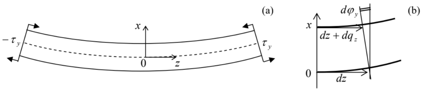Figure 7.8. Rod bending, in a local reference frame (specific for each cross-section).

Just as in the tensile stress experiment (Figure 6), the components of the stress forces \(d \mathbf{F}\), normal to the rod length, have to equal zero on the surface of the rod. Repeating the arguments made for the tensile stress discussion, we have to conclude that only one diagonal component of the tensor (in Figure 8 , \(\sigma_{z z}\) ) may differ from zero: \[\sigma_{i j^{\prime}}=\delta_{j z} \sigma_{z z} .\] However, in contrast to the tensile stress, at pure static bending, the net force directed along the rod has to vanish: \[F_{z}=\int_{S} \sigma_{z z} d^{2} r=0,\] where \(S\) is the rod’s cross-section, so that \(\sigma_{z z}\) has to change its sign at some point of the \(x\)-axis (in Figure 8, selected to lie in the plane of the bent rod). Thus, the bending deformation may be viewed as a combination of stretching some layers of the rod (bottom layers in Figure 8) with compression of other (top) layers.

Since it is hard to make more immediate conclusions about the stress distribution, let us turn over to strain, assuming that the rod’s cross-section is virtually constant on the length of our local analysis. From the above representation of bending as a combination of stretching and compression, it evident that the longitudinal deformation \(q_{z}\) has to vanish along some neutral line on the rod’s crosssection - in Figure 8, represented by the dashed line. \({ }^{28}\) Selecting the origin of the \(x\)-coordinate on this line, and expanding the relative deformation in the Taylor series in \(x\), due to the cross-section smallness we may keep just the first, linear term: \[s_{z z} \equiv \frac{d q_{z}}{d z}=-\frac{x}{R} .\] The constant \(R\) has the sense of the curvature radius of the bent rod. Indeed, on a small segment \(d z\), the cross-section turns by a small angle \(d \varphi_{y}=-d q_{z} / x\) (Figure 8b). Using Eq. (66), we get \(d \varphi_{y}=d z / R\), which is the usual definition of the curvature radius \(R\) in the differential geometry, for our special choice of the coordinate axes. \({ }^{29}\)Expressions for other components of the strain tensor are harder to guess (like at the tensile stress, not all of them are equal to zero!), but what we already know about \(\sigma_{z z}\) and \(S_{z z}\) is already sufficient to start formal calculations. Indeed, plugging Eq. (64) into Hooke’s law in the form (49b), and comparing the result for \(s_{z z}\) with Eq. (66), we find \[\sigma_{z z}=-E \frac{x}{R}\] From the same Eq. (49b), we could also find the transverse components of the strain tensor, and conclude that they are related to \(s_{z z}\) exactly as at the tensile stress: \[s_{x x}=s_{y y}=-v s_{z z},\] and then, integrating these relations along the cross-section of the rod, find the deformation of the crosssection’s shape. More important for us, however, is the calculation of the relation between the rod’s curvature and the net torque acting on a given cross-section \(S\) (taking \(d A_{z}>0\) ): \[\tau_{y} \equiv \int_{S}(\mathbf{r} \times d \mathbf{F})_{y}=-\int_{S} x \sigma_{z z} d^{2} r=\frac{E}{R} \int_{S} x^{2} d^{2} r=\frac{E I_{y}}{R},\] where \(I_{y}\) is a geometric constant defined as \[I_{y} \equiv \int_{S} x^{2} d x d y .\] Note that this factor, defining the bending rigidity of the rod, grows as fast as \(a^{4}\) with the linear scale \(a\) of the cross-section. \({ }^{30}\)

In these expressions, \(x\) has to be counted from the neutral line. Let us see where exactly does this line pass through the rod’s cross-section. Plugging the result (67) into Eq. (65), we get the condition defining the neutral line: \[\int_{S} x d x d y=0\] This condition allows a simple interpretation. Imagine a thin sheet of some material, with a constant mass density \(\sigma\) per unit area, cut in the form of the rod’s cross-section. If we place a reference frame into its center of mass, then, by its definition, \[\sigma \int_{S} \mathbf{r} d x d y=0\] Comparing this condition with Eq. (71), we see that one of the neutral lines has to pass through the center of mass of the sheet, which may be called the "center of mass of the cross-section". Using the same analogy, we see that the integral \(I_{y}\) given by Eq. (72) may be interpreted as the moment of inertia of the same imaginary sheet of material, with \(\sigma\) formally equal to 1 , for its rotation about the neutral line - cf. Eq. (4.24). This analogy is so convenient that the integral is usually called the moment of inertia of the cross-section and denoted similarly - just as has been done above. So, our basic result (69) may be re-written as \[\frac{1}{R}=\frac{\tau_{y}}{E I_{y}} .\] This relation is only valid if the deformation is small in the sense \(R \gg a\). Still, since the deviations of the rod from its unstrained shape may accumulate along its length, Eq. (73) may be used for calculations of large "global" deviations of the rod from equilibrium, on a length scale much larger than \(a\). To describe such deformations, Eq. (73) has to be complemented by conditions of the balance of the bending forces and torques. Unfortunately, this requires a bit more differential geometry than I have time for, and I will only discuss this procedure for the simplest case of relatively small transverse deviations \(q \equiv q_{x}\) of the rod from its initial straight shape, which will be used for the \(z\)-axis (Figure 9a), for example by some bulk-distributed force \(\mathbf{f}=\mathbf{n}_{x} f_{x}(z)\). (The simplest example is a uniform gravity field, for which \(f_{x}=-\rho g=\) const.) Note that in the forthcoming discussion the reference frame will be global, i.e. common for the whole rod, rather than local (pertaining to each cross-section) as it was in the previous analysis - cf. Figure 8 .

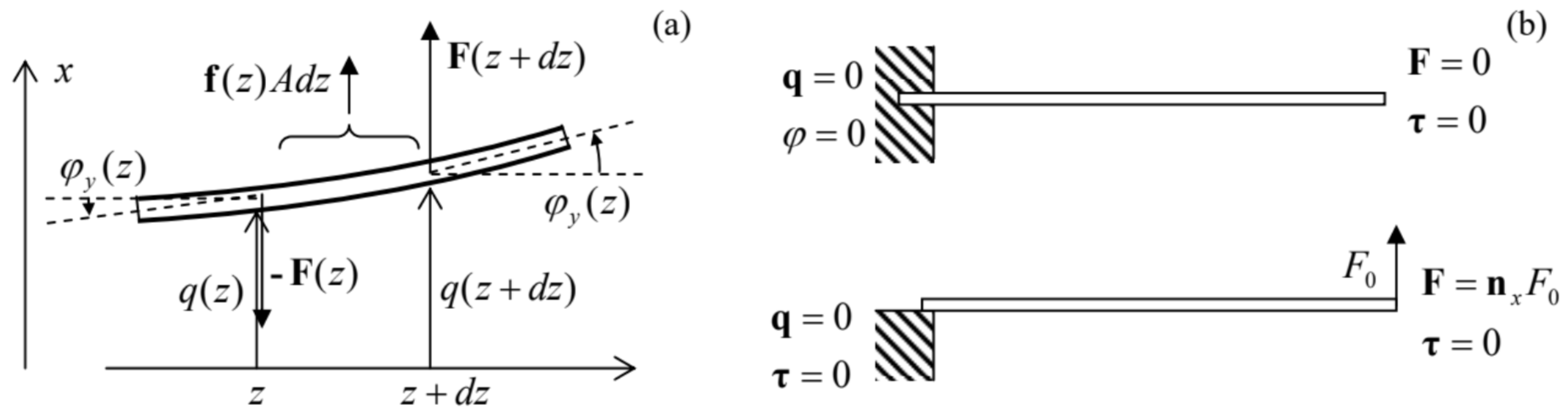Figure 7.9. A global picture of rod bending: (a) the forces acting on a small fragment of a rod, and (b) two bending problem examples, each with two typical but different boundary conditions.

First of all, we may write a differential static relation for the average vertical force \(\mathbf{F}=\mathbf{n}_{x} F_{x}(z)\) exerted on the part of the rod located to the left of its cross-section - located at point \(z\). This relation expresses the balance of vertical forces acting on a small fragment \(d z\) of the rod (Figure 9a), necessary for the absence of its linear acceleration: \(F_{x}(z+d z)-F_{x}(z)+f_{x}(z) A d z=0\), giving \[\frac{d F_{x}}{d z}=-f_{x} A,\] where \(A\) is the cross-section area. Note that this vertical component of the internal forces has been neglected at our derivation of Eq. (73), and hence our final results will be valid only if the ratio \(F_{x} / A\) is much smaller than the magnitude of \(\sigma_{z z}\) described by Eq. (67). However, these forces create the very torque \(\tau=\mathbf{n}_{y} \tau_{y}\) that causes the bending, and thus have to be taken into account at the analysis of the global picture. Such account may be made by writing the balance of torque components, acting on the same rod fragment of length \(d z\), necessary for the absence of its angular acceleration: \(d \tau_{y}+F_{x} d z=0\), giving \[\frac{d \tau_{y}}{d z}=-F_{x} .\] These two equations should be complemented by two geometric relations. The first of them is \(d \varphi_{y} / d z=1 / R\), which has already been discussed above. We may immediately combine it with the basic result \((73)\) of the local analysis, getting: \[\frac{d \varphi_{y}}{d z}=\frac{\tau_{y}}{E I_{y}} .\] The final equation is the geometric relation evident from Figure 9a: \[\frac{d q_{x}}{d z}=\varphi_{y},\] which is (as all expressions of our simple analysis) only valid for small bending angles, \(\left|\varphi_{y}\right|<<1 .\) The four differential equations (74)-(77) are sufficient for the full solution of the weak bending problem, if complemented by appropriate boundary conditions. Figure \(9 \mathrm{~b}\) shows the conditions most frequently met in practice. Let us solve, for example, the problem shown on the top panel of Figure \(9 \mathrm{~b}\) : bending of a rod, "clamped" at one end (say, immersed into a rigid wall), under its own weight. Considering, for the sake of simplicity, a uniform rod, \({ }^{31}\) we may integrate these equations one by one, each time using the appropriate boundary conditions. To start, Eq. (74) with \(f_{x}=-\rho g\) yields \[F_{x}=\rho g A z+\text { const }=\rho g A(z-l),\] where the integration constant has been selected to satisfy the right-end boundary condition: \(F_{x}=0\) at \(z\) \(=l\). As a sanity check, at the left wall \((z=0), F_{x}=-\rho g A l=-m g\), meaning that the whole weight of the rod is exerted on the wall - fine.

Next, plugging Eq. (78) into Eq. (75) and integrating, we get \[\tau_{y}=-\frac{\rho g A}{2}\left(z^{2}-2 l z\right)+\text { const }=-\frac{\rho g A}{2}\left(z^{2}-2 l z+l^{2}\right) \equiv-\frac{\rho g A}{2}(z-l)^{2},\] where the integration constant’s choice ensures the second right-boundary condition: \(\tau_{y}=0\) at \(z=l-\) see Figure \(9 \mathrm{~b}\) again. Now proceeding in the same fashion to Eq. (76), we get \[\varphi_{y}=-\frac{\rho g A}{2 E I_{y}} \frac{(z-l)^{3}}{3}+\text { const }=-\frac{\rho g A}{6 E I_{y}}\left[(z-l)^{3}+l^{3}\right],\] where the integration constant is selected to satisfy the clamping condition at the left end of the rod: \(\varphi_{y}\) \(=0\) at \(z=0\). (Note that this is different from the support condition illustrated on the lower panel of Figure \(9 \mathrm{~b}\), which allows the angle at \(z=0\) to be different from zero, but requires the torque to vanish.) Finally, integrating Eq. (77) with \(\varphi_{y}\) given by Eq. (80), we get the rod’s global deformation law, \[q_{x}(z)=-\frac{\rho g A}{6 E I_{y}}\left[\frac{(z-l)^{4}}{4}+l^{3} z+\mathrm{const}\right]=-\frac{\rho g A}{6 E I_{y}}\left[\frac{(z-l)^{4}}{4}+l^{3} z-\frac{l^{4}}{4}\right],\] where the integration constant is selected to satisfy the second left-boundary condition: \(q=0\) at \(z=0\). So, the bending law is sort of complicated even in this very simple problem. It is also remarkable how fast does the end’s displacement grow with the increase of the rod’s length: \[q_{x}(l)=-\frac{\rho g A l^{4}}{8 E I_{y}} .\] To conclude the solution, let us discuss the validity of this result. First, the geometric relation (77) is only valid if \(\left|\varphi_{y}(l)\right|<<1\), and hence if \(\left|q_{x}(l)\right|<<l\). Next, the local formula Eq. (76) is valid if \(1 / R\) \(=\tau(l) / E I_{y}<<1 / a \sim A^{-1 / 2}\). Using the results (79) and (82), we see that the latter condition is equivalent to \(\left|q_{x}(l)\right|<<l^{2} / a\), i.e. is weaker than the former one, because all our analysis has been based on the assumption \(l>>a\).

Another point of concern may be that the off-diagonal stress component \(\sigma_{x z} \sim F_{x} / A\), which is created by the vertical gravity forces, has been ignored in our local analysis. For that approximation to be valid, this component must be much smaller than the diagonal component \(\sigma_{z z} \sim a E / R=a \tau / I_{y}\) taken into account in that analysis. Using Eqs. (78) and (80), we are getting the following estimates: \(\sigma_{x z} \sim \rho g l\), \(\sigma_{z z} \sim a \rho g A l^{2} / I_{y} \sim a^{3} \rho g l^{2} / I_{y}\). According to its definition \((70), I_{y}\) may be crudely estimated as \(a^{4}\), so that we finally get the simple condition \(a<<l\), which has been assumed from the very beginning of our solution.

---

\({ }^{27}\) For its review see, e.g., Secs. 11-15 in L. Landau and E. Lifshitz, Theory of Elasticity, \(3^{\text {rd }}\) ed., ButterworthHeinemann, \(1986 .\)

\({ }^{28}\) Strictly speaking, that dashed line is the intersection of the neutral surface (the continuous set of such neutral lines for all cross-sections of the rod) with the plane of the drawing.

\({ }_{29}\) Indeed, for \((d x / d z)^{2}<<1\), the general formula MA Eq. (4.3) for the curvature (with the appropriate replacements \(f \rightarrow x\) and \(x \rightarrow z\) ) is reduced to \(1 / R=d^{2} x / d z^{2}=d(d x / d z) / d z=d\left(\tan \varphi_{y}\right) / d z \approx d \varphi_{y} / d z\).

\({ }^{30}\) In particular, this is the reason why the usual electric wires are made not of a solid copper core, but rather a twisted set of thinner sub-wires, which may slip relative to each other, increasing the wire flexibility.

\({ }^{31}\) As should be clear from their derivation, Eqs. (74)-(77) are valid for any distribution of parameters \(A, E, I_{y}\), and \(\rho\) over the rod’s length, provided that the rod is quasi-uniform, i.e. its parameters’ changes are so slow that the local relation (76) is still valid at any point.