9.2: Chaos in Dynamic Systems

Proceeding to the discussion of chaos in dynamic systems, it is more natural, with our background, to illustrate this discussion not with the Lorenz Eqs. (1), but with the system of equations describing a dissipative pendulum driven by a sinusoidal external force, which was repeatedly discussed in Chapter 5. Introducing two new variables, the normalized momentum \(p \equiv(d q / d t) / \omega_{0}\), and the external force’s full phase \(\psi \equiv \omega t\), we may rewrite Eq. (5.42) describing the pendulum, in a form similar to Eq. (1), i.e. as a system of three first-order ordinary differential equations: \[\begin{aligned} &\dot{q}=\omega_{0} p, \\ &\dot{p}=-\omega_{0} \sin q-2 \delta p+\left(f_{0} / \omega_{0}\right) \cos \psi, \\ &\dot{\psi}=\omega . \end{aligned}\] Figure 4 several results of a numerical solution of Eq. (10). \({ }^{10}\) In all cases, parameters \(\delta, \omega_{0}\), and \(f_{0}\) are fixed, while the external frequency \(\omega\) is gradually changed. For the case shown on the top panel, the system still tends to a stable periodic solution, with very low contents of higher harmonics. If the external force frequency is reduced by a just few percent, the \(3^{\text {rd }}\) subharmonic may be excited. (This effect has already been discussed in Sec. \(5.8\) - see, e.g., Figure 5.15.) The next panel shows that just a small further reduction of the frequency \(\omega\) leads to a new tripling of the period, i.e. the generation of a complex waveform with the \(9^{\text {th }}\) subharmonic. Finally (see the bottom panel of Figure 4), even a minor further change of \(\omega\) leads to oscillations without any visible period, e.g., to the chaos.

In order to trace this transition, a direct inspection of the oscillation waveforms \(q(t)\) is not very convenient, and trajectories on the phase plane \([q, p]\) also become messy if plotted for many periods of the external frequency. In situations like this, the Poincaré (or "stroboscopic") plane, already discussed in Sec. 5.6, is much more useful. As a reminder, this is essentially just the phase plane \([q, p]\), but with the points highlighted only once a period, e.g., at \(\psi=2 \pi n\), with \(n=1,2, \ldots\) On this plane, periodic oscillations of frequency \(\omega\) are represented just as one fixed point - see, e.g. the top panel in the right column of Figure 4. The \(3^{\text {rd }}\) subharmonic generation, shown on the next panel, means the oscillation period’s tripling and is reflected on the Poincaré plane as splitting of the fixed point into three. It is evident that this transition is similar to the period-doubling bifurcation in the logistic map, besides the fact (already discussed in Sec. 5.8) that in systems with an antisymmetric nonlinearity, such as the pendulum (10), the \(3^{\text {rd }}\) subharmonic is easier to excite. From this point, the \(9^{\text {th }}\) harmonic generation (shown on the \(3^{\text {rd }}\) panel of Figure 4), i.e. one more splitting of the points on the Poincare plane, may be understood as one more step on the Feigenbaum-like route to chaos - see the bottom panel of that figure.

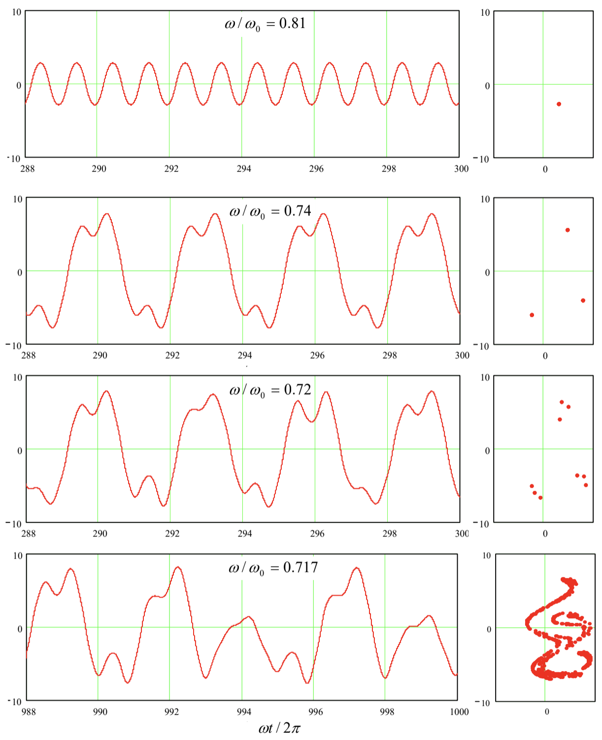
Figure 9.4. Oscillations in a pendulum with weak damping, \(\delta / \omega_{0}=0.1\), driven by a sinusoidal external force with a fixed effective amplitude \(f_{0} / \omega_{0}{ }^{2}=1\), and several close values of the frequency \(\omega\) (listed on the panels). Left panel column: the oscillation waveforms \(q(t)\) recorded after certain initial transient intervals. Right column: representations of the same processes on the Poincaré plane of the variables \([q, p]\), with the \(q\)-axis turned vertically, for the convenience of comparison with the left panels. So, the transition to chaos in dynamic systems may be at least qualitatively similar to than in 1D maps, with a law similar to Eq. (6) for the critical values of some parameter of the system (in Figure 4, frequency \(\omega\) ), though with a system-specific value of the coefficient \(\delta\). Moreover, we may consider the first two differential equations of the system (10) as a 2D map that relates the vector \(\left\{q_{n+1}, p_{n+1}\right\}\) of the coordinate and momentum, measured at \(\psi=2 \pi(n+1)\), with the previous value \(\left\{q_{n}, p_{n}\right\}\) of that vector, reached at \(\psi=2 \pi n\).

Unfortunately, this similarity also implies that the deterministic chaos in dynamic systems is at least as complex, and is as little understood, as in maps. For example, Figure 5 shows (a part of) the phase diagram of the externally-driven pendulum, with the red bar marking the route to chaos traced in Figure 4 , and shading/hatching styles marking different oscillation regimes. One can see that the pattern is at least as complex as that shown in Figs. 2 and 3, and, besides a few features, \({ }^{11}\) is equally unpredictable from the form of the equation.

 

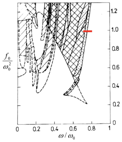
Figure 9.5. The phase diagram of an externally-driven pendulum with weak damping \(\left(\delta / \omega_{0}=0.1\right)\). The regions of oscillations with the basic period are not shaded; the notation for other regions is as follows. Doted: subharmonic generation; cross-hatched: chaos; hatched: either chaos or the basic period (depending on the initial conditions); hatch-dotted: either the basic period or subharmonics. Solid lines show the boundaries of single-regime regions, while dashed lines are the boundaries of the regions where several types of motion are possible. (Figure courtesy V. Kornev.)

Are there any valuable general results concerning the deterministic chaos in dynamic systems? The most important (though an almost evident) result is that this phenomenon is impossible in any system described by one or two first-order differential equations with time-independent right-hand sides. Indeed, let us start with a single equation \[\dot{q}=f(q),\] where \(f(q)\) is any single-valued function. This equation may be directly integrated to give \[t=\int^{q} \frac{d q^{\prime}}{f\left(q^{\prime}\right)}+\text { const },\] showing that the relation between \(q\) and \(t\) is unique and hence does not leave any place for chaos.

Next, let us explore a system of two such equations: \[\begin{aligned} &\dot{q}_{1}=f_{1}\left(q_{1}, q_{2}\right), \\ &\dot{q}_{2}=f_{2}\left(q_{1}, q_{2}\right) . \end{aligned}\] Consider its phase plane shown schematically in Figure 6. In a "usual" system, the trajectories approach either some fixed point (Figure 6a) describing static equilibrium, or a limit cycle (Figure 6b) describing periodic oscillations. (Both notions are united by the term attractor because they "attract" trajectories launched from various initial conditions.) On the other hand, phase plane trajectories of a chaotic system of equations that describe physical variables (which cannot be infinite), should be confined to a limited phase plane area, and simultaneously cannot start repeating each other. (This topology is frequently called the strange attractor.) For that, the 2D trajectories need to cross - see, e.g., point A in Figure \(6 \mathrm{c}\).

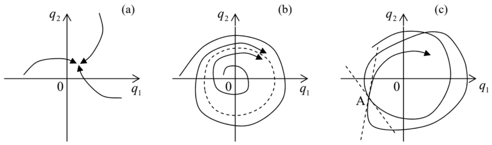
Figure 9.6. Attractors in dynamical systems: (a) a fixed point, (b) a limit cycle, and (c) a strange attractor.

However, in the case described by Eqs. (13), such a crossing is clearly impossible, because according to these equations, the tangent of a phase plane trajectory is a unique function of the coordinates \(\left\{q_{1}, q_{2}\right\}\) : \[\frac{d q_{1}}{d q_{2}}=\frac{f_{1}\left(q_{1}, q_{2}\right)}{f_{2}\left(q_{1}, q_{2}\right)} .\] Thus, in this case the deterministic chaos is impossible. \({ }^{12}\) It becomes, however, readily possible if the right-hand sides of a system similar to Eq. (13) depend either on other variables of the system or time. For example, if we consider the first two differential equations of the system (10), in the case \(f_{0}=0\) they have the structure of the system (13) and hence the chaos is impossible, even at \(\delta<0\) when (as we know from Sec. 5.4) the system allows self-excitation of oscillations - leading to a limit-cycle attractor. However, if \(f_{0} \neq 0\), this argument does not work any longer, and (as we have already seen) the system may have a strange attractor - which is, for dynamic systems, a synonym for the deterministic chaos.

Thus, chaos is only possible in autonomous dynamic systems described by three or more differential equations of the first order. \({ }^{13}\)

---

\({ }^{10}\) In the actual simulation, a small term \(\varepsilon q\), with \(\varepsilon<1\), has been added to the left-hand side of this equation. This term slightly tames the trend of the solution to spread along the \(q\)-axis, and makes the presentation of results easier, without affecting the system’s dynamics too much.

\({ }^{11}\) In some cases, it is possible to predict a parameter region where chaos cannot happen, due to the lack of any instability-amplification mechanism. Unfortunately, typically the analytically predicted boundaries of such a region form a rather loose envelope of the actual (numerically simulated) chaotic regions.

\({ }^{12}\) A mathematically strict formulation of this statement is called the Poincare-Bendixon theorem, which was proved by Ivar Bendixon as early as in \(1901 .\)

\({ }^{13}\) Since a typical dynamic system with one degree of freedom is described by two such equations, the number of first-order equations describing a dynamic system is sometimes called the number of its half-degrees of freedom. This notion is very useful and popular in statistical mechanics - see, e.g., SM Sec. \(2.2\) and on.