10.2: Adiabatic Invariance

One more application of the Hamiltonian formalism in classical mechanics is the solution of the following problem. \({ }^{9}\) Earlier in the course, we already studied some effects of time variation of parameters of a single oscillator (Sec. 5.5) and coupled oscillators (Sec. 6.5). However, those discussions were focused on the case when the parameter variation speed is comparable with the own oscillation frequency (or frequencies) of the system. Another practically important case is when some system’s parameter (let us call it \(\lambda\) ) is changed much more slowly (adiabatically \(^{10}\) ), \[\left|\frac{\dot{\lambda}}{\lambda}\right|<<\frac{1}{T},\] where \(\tau\) is a typical period of oscillations in the system. Let us consider a 1D system whose Hamiltonian \(H(q, p, \lambda)\) depends on time only via such a slow evolution of such parameter \(\lambda=\lambda(t)\), and whose initial energy restricts the system’s motion to a finite coordinate interval - see, e.g., Figure 3.2c.

Then, as we know from Sec. 3.3, if the parameter \(\lambda\) is constant, the system performs a periodic (though not necessarily sinusoidal) motion back and forth the \(q\)-axis, or, in a different language, along a closed trajectory on the phase plane \([q, p]\) - see Figure \(1 .{ }^{11}\) According to Eq. (8), in this case \(H\) is constant along the trajectory. (To distinguish this particular value from the Hamiltonian function as such, I will call it \(E\), implying that this constant coincides with the full mechanical energy \(E-\) as does for the Hamiltonian (10), though this assumption is not necessary for the calculation made below.)

The oscillation period \(T\) may be calculated as a contour integral along this closed trajectory: \[\tau \equiv \int_{0}^{\tau} d t=\oint \frac{d t}{d q} d q \equiv \oint \frac{1}{\dot{q}} d q .\] Using the first of the Hamilton equations (7), we may represent this integral as \[\tau=\oint \frac{1}{\partial H / \partial p} d q .\] At each given point \(q, H=E\) is a function of \(p\) alone, so that we may flip the partial derivative in the denominator just as the full derivative, and rewrite Eq. (30) as \[\tau=\oint \frac{\partial p}{\partial E} d q \text {. }\] For the particular Hamiltonian (10), this relation is immediately reduced to Eq. (3.27), now in the form of a contour integral: \[\tau=\left(\frac{m_{\mathrm{ef}}}{2}\right)^{1 / 2} \oint \frac{1}{\left[E-U_{\mathrm{ef}}(q)\right]^{1 / 2}} d q\] 

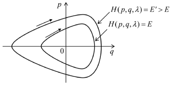
Fig. 10.1. Phase-plane representation of periodic oscillations of a 1D Hamiltonian system, for two values of energy (schematically).

Naively, it may look that these formulas may be also used to find the motion period’s change when the parameter \(\lambda\) is being changed adiabatically, for example, by plugging the given functions \(m_{\mathrm{ef}}(\lambda)\) and \(U_{\mathrm{ef}}(q, \lambda)\) into Eq. (32). However, there is no guarantee that the energy \(E\) in that integral would stay constant as the parameter changes, and indeed we will see below that this is not necessarily the case. Even more interestingly, in the most important case of the harmonic oscillator \(\left(U_{\mathrm{ef}}=\kappa_{\mathrm{ef}} q^{2} / 2\right)\), whose oscillation period \(\tau\) does not depend on \(E\) (see Eq. (3.29) and its discussion), its variation in the adiabatic limit (28) may be readily predicted: \(\tau(\lambda)=2 \pi / \omega_{0}(\lambda)=2 \pi\left[m_{\mathrm{ef}}(\lambda) / \kappa_{\mathrm{ef}}(\lambda)\right]^{1 / 2}\), but the dependence of the oscillation energy \(E\) (and hence the oscillation amplitude) on \(\lambda\) is not immediately obvious.

In order to address this issue, let us use Eq. (8) (with \(E=H\) ) to represent the rate of the energy change with \(\lambda(t)\), i.e. in time, as \[\frac{d E}{d t}=\frac{\partial H}{\partial t}=\frac{\partial H}{\partial \lambda} \frac{d \lambda}{d t} .\] Since we are interested in a very slow (adiabatic) time evolution of energy, we can average Eq. (33) over fast oscillations in the system, for example over one oscillation period \(T\), treating \(d \lambda / d t\) as a constant during this averaging. (This is the most critical point of this argumentation, because at any non- vanishing rate of parameter change the oscillations are, strictly speaking, non-periodic. \({ }^{12}\) ) The averaging yields \[\overline{\frac{d E}{d t}}=\frac{d \lambda}{d t} \frac{\overline{\partial H}}{\partial \lambda} \equiv \frac{d \lambda}{d t} \frac{1}{\tau} \int_{0}^{\tau} \frac{\partial H}{\partial \lambda} d t .\] Transforming this time integral to the contour one, just as we did at the transition from Eq. (29) to Eq. (30), and then using Eq. (31) for \(\tau\), we get \[\frac{\overline{d E}}{d t}=\frac{d \lambda}{d t} \frac{\oint \frac{\partial H / \partial \lambda}{\partial H / \partial p} d q}{\oint \frac{\partial p}{\partial E} d q}\] At each point \(q\) of the contour, \(H\) is a function of not only \(\lambda\), but also of \(p\), which may be also \(\lambda\) dependent, so that if \(E\) is fixed, the partial differentiation of the relation \(E=H\) over \(\lambda\) yields \[\frac{\partial H}{\partial \lambda}+\frac{\partial H}{\partial p} \frac{\partial p}{\partial \lambda}=0, \text { i.e. } \frac{\partial H / \partial \lambda}{\partial H / \partial p}=-\frac{\partial p}{\partial \lambda} .\] Plugging the last relation to Eq.(35), we get \[\frac{\overline{d E}}{d t}=-\frac{d \lambda}{d t} \frac{\oint \frac{\partial p}{\partial \lambda} d q}{\oint \frac{\partial p}{\partial E} d q}\] Since the left-hand side of Eq. (37) and the derivative \(d \lambda / d t\) do not depend on \(q\), we may move them into the integrals over \(q\) as constants, and rewrite Eq. (37) as \[\oint\left(\frac{\partial p}{\partial E} \frac{\overline{d E}}{d t}+\frac{\partial p}{\partial \lambda} \frac{d \lambda}{d t}\right) d q=0 .\] Now let us consider the following integral over the same phase-plane contour, \[J \equiv \frac{1}{2 \pi} \oint p d q,\] called the action variable. Just to understand its physical sense, let us calculate \(J\) for a harmonic oscillator (14). As we know very well from Chapter 5, for such an oscillator, \(q=A \cos \Psi, p=-\) \(m_{\text {ef }} \omega_{0} A \sin \Psi\) (with \(\Psi=\omega_{0} t+\) const), so that \(J\) may be easily expressed either via the oscillations’ amplitude \(A\), or via their energy \(E=H=m_{\mathrm{ef}} \omega_{0}^{2} A^{2} / 2\) : \[J=\frac{1}{2 \pi} \oint p d q=\frac{1}{2 \pi} \int_{\Psi=0}^{\Psi=2 \pi}\left(-m_{\mathrm{ef}} \omega_{0} A \sin \Psi\right) d(A \cos \Psi)=\frac{m_{\mathrm{ef}} \omega_{0}}{2} A^{2}=\frac{E}{\omega_{0}} .\] Returning to a general system with adiabatically changed parameter \(\lambda\), let us use the definition of \(J\), Eq. (39), to calculate its time derivative, again taking into account that at each point \(q\) of the trajectory, \(p\) is a function of \(E\) and \(\lambda\) : \[\frac{d J}{d t}=\frac{1}{2 \pi} \oint \frac{d p}{d t} d q=\frac{1}{2 \pi} \oint\left(\frac{\partial p}{\partial E} \frac{d E}{d t}+\frac{\partial p}{\partial \lambda} \frac{d \lambda}{d t}\right) d q .\] Within the accuracy of our approximation, in which the contour integrals (38) and (41) are calculated along a closed trajectory, the factor \(d E / d t\) is indistinguishable from its time average, and these integrals coincide so that the result (38) is applicable to Eq. (41) as well. Hence, we have finally arrived at a very important result: at a slow parameter variation, \(d J / d t=0\), i.e. the action variable remains constant: \[J=\text { const }\] This is the famous adiabatic invariance. \({ }^{13}\) In particular, according to Eq. (40), in a harmonic oscillator, the energy of oscillations changes proportionately to its own (slowly changed) frequency.Before moving on, let me briefly note that the adiabatic invariance is not the only application of the action variable \(J\). Since the initial choice of generalized coordinates and velocities (and hence the generalized momenta) in analytical mechanics is arbitrary (see Sec. 2.1), it is almost evident that \(J\) may be taken for a new generalized momentum corresponding to a certain new generalized coordinate \(\Theta,{ }^{14}\) and that the pair \(\{J, \Theta\}\) should satisfy the Hamilton equations (7), in particular, \[\frac{d \Theta}{d t}=\frac{\partial H}{\partial J} .\] Following the commitment of Sec. 1 (made there for the "old" arguments \(q_{j}, p_{j}\) ), before the differentiation on the right-hand side of Eq. (43), \(H\) should be expressed as a function (besides \(t\) ) of the "new" arguments \(J\) and \(\Theta\). For time-independent Hamiltonian systems, \(H\) is uniquely defined by \(J-\) see, e.g., Eq. (40). Hence in this case the right-hand side of Eq. (43) does not depend on either \(t\) or \(\Theta\), so that according to that equation, \(\Theta\) (called the angle variable) is a linear function of time: \[\Theta=\frac{\partial H}{\partial J} t+\text { const } .\] For a harmonic oscillator, according to Eq. (40), the derivative \(\partial H / \partial J=\partial E / \partial J\) is just \(\omega_{0} \equiv 2 \pi / T\), so that \(\Theta=\omega_{0} t+\) const, i.e. it is just the full phase \(\Psi\) that was repeatedly used in this course \(-\) especially in Chapter 5 . It may be shown that a more general form of this relation, \[\frac{\partial H}{\partial J}=\frac{2 \pi}{\tau},\] is valid for an arbitrary system described by Eq. (10). Thus, Eq. (44) becomes \[\Theta=2 \pi \frac{t}{\tau}+\text { const } \text {. }\] This means that for an arbitrary (nonlinear) 1D oscillator, the angle variable \(\Theta\) is a convenient generalization of the full phase \(\Psi\). Due to this reason, the variables \(J\) and \(\Theta\) present a convenient tool for discussion of certain fine points of the dynamics of strongly nonlinear oscillators - for whose discussion I, unfortunately, do not have time/space. \({ }^{15}\)

---

\({ }_{9}\) Various aspects of this problem and its quantum-mechanical extensions were first discussed by L. Le Cornu (1895), Lord Rayleigh (1902), H. Lorentz (1911), P. Ehrenfest (1916), and M. Born and V. Fock (1928).

\({ }_{10}\) This term is also used in thermodynamics and statistical mechanics, where it implies not only a slow parameter variation (if any) but also thermal insulation of the system - see, e.g., SM Sec. 1.3. Evidently, the latter condition is irrelevant in our current context.

\({ }^{11}\) In Sec. 5.6, we discussed this plane for the particular case of sinusoidal oscillations - see Figure \(5.9\)

\({ }^{12}\) Because of the implied nature of this conjecture (which is very close to the assumptions made at the derivation of the reduced equations in Sec. 5.3), new, more strict (but also much more cumbersome) proofs of the final Eq. (42) are still being offered in literature - see, e.g., C. Wells and S. Siklos, Eur. J. Phys. 28, 105 (2007) and/or A. Lobo et al., Eur. J. Phys. 33, 1063 (2012).

\({ }^{13}\) For certain particular oscillators, e.g., a point pendulum, Eq. (42) may be also proved directly - an exercise highly recommended to the reader.

\({ }_{14}\) This, again, is a plausible argument but not a strict proof. Indeed: though, according to its definition (39), \(J\) is nothing more than a sum of several (formally, the infinite number of) values of the momentum \(p\), they are not independent, but have to be selected on the same closed trajectory on the phase plane. For more mathematical vigor, the reader is referred to Sec. 45 of Mechanics by Landau and Lifshitz (which was repeatedly cited above), which discusses the general rules of the so-called canonical transformations from one set of Hamiltonian arguments to another one - say from \(\{p, q\}\) to \(\{J, \Theta\}\).

\({ }^{15}\) An interested reader may be referred, for example, to Chapter 6 in J. Jose and E. Saletan, Classical Dynamics, Cambridge U. Press, \(1998 .\)