4.4: Limit Cycles

Poincaré-Bendixson theorem

Coupled first-order differential equations in two dimensions of the form

\[\dot{x} = f(x,y)\hspace{0.55in}\dot{y} = g(x,y) \label{4.10}\]

occur frequently in physics. The state-space paths do not cross for such two-dimensional autonomous systems, where an autonomous system is not explicitly dependent on time.

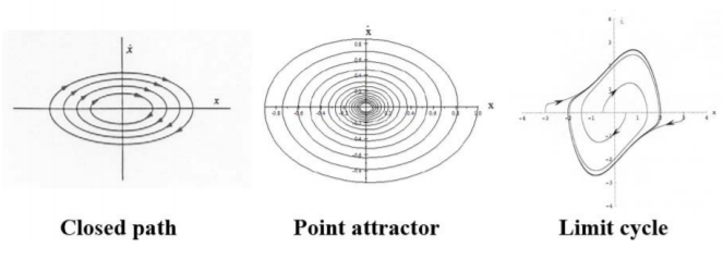
The Poincaré-Bendixson theorem states that, state-space, and phase-space, can have three possible paths:

1. closed paths, like the elliptical paths for the undamped harmonic oscillator,
2. terminate at an equilibrium point as \(t\rightarrow \infty\), like the point attractor for a damped harmonic oscillator,
3. tend to a limit cycle as \(t\rightarrow \infty\).

The limit cycle is unusual in that the periodic motion tends asymptotically to the limit-cycle attractor independent of whether the initial values are inside or outside the limit cycle. The balance of dissipative forces and driving forces often leads to limit-cycle attractors, especially in biological applications. Identification of limit-cycle attractors, as well as the trajectories of the motion towards these limit-cycle attractors, is more complicated than for point attractors.

Figure \(\PageIndex{1}\): The Poincaré-Bendixson theorem allows the following three scenarios for two-dimensional autonomous systems. (1) Closed paths as illustrated by the undamped harmonic oscillator. (2) Terminate at an equilibrium point as \(t\rightarrow \infty\), as illustrated by the damped harmonic oscillator, and (3) Tend to a limit cycle as \(t\rightarrow \infty\) as illustrated by the van der Pol oscillator.

van der Pol damped harmonic oscillator

The van der Pol damped harmonic oscillator illustrates a non-linear equation that leads to a well-studied, limit-cycle attractor that has important applications in diverse fields. The van der Pol oscillator has an equation of motion given by

\[\frac{d^{2}x}{dt^{2}}+\mu \left( x^{2}-1\right) \frac{dx}{dt}+\omega _{0}^{2}x = 0 \label{4.11}\]

The non-linear \(\mu \left( x^{2}-1\right) \frac{dx}{dt}\) damping term is unusual in that the sign changes when \(x = 1\) leading to positive damping for \( x>1\) and negative damping for \(x<1.\) To simplify Equation \ref{4.11}, assume that the term \(\omega _{0}^{2}x = x,\) that is, \(\omega _{0}^{2} = 1\).

This equation was studied extensively during the 1920’s and 1930’s by the Dutch engineer, Balthazar van der Pol, for describing electronic circuits that incorporate feedback. The form of the solution can be simplified by defining a variable \(y\equiv \frac{dx}{dt}.\) Then the second-order Equation \ref{4.11} can be expressed as two coupled first-order equations.

\[y \equiv \frac{dx}{dt} \label{4.12}\]

\[ \frac{dy}{dt} = -x-\mu \left( x^{2}-1\right) y \label{4.13}\]

It is advantageous to transform the \(\left( \dot{x},x\right)\) state space to polar coordinates by setting

\[\begin{align} x & = &r\cos \theta \label{4.14}\\ y & = &r\sin \theta \nonumber \end{align}\]

and using the fact that \(\ r^{2} = x^{2}+y^{2}\). Therefore

\[r\frac{dr}{dt} = x\frac{dx}{dt}+y\frac{dy}{dt}\label{4.15}\]

Similarly for the angle coordinate

\[\frac{dx}{dt} = \frac{dr}{dt}\cos \theta -r\frac{d\theta }{dt}\sin \theta \label{4.16}\]

\[\frac{dy}{dt} = \frac{dr}{dt}\sin \theta +r\frac{d\theta }{dt}\cos \theta \label{4.17}\]

Figure \(\PageIndex{2}\): Solutions of the van der Pol system for \(\mu = 0.2\) top row and \(\mu = 5\) bottom row, assuming that \(\omega^2_0 = 1\). The left column shows the time dependence \(x(t)\). The right column shows the corresponding \((x,\dot{x})\) state space plots. Upper: Weak nonlinearity, \(\mu = \mathbf{0.2}\); At large times the solution tends to one limit cycle for initial values inside or outside the limit cycle attractor. The amplitude \(x(t)\) for two initial conditions approaches an approximately harmonic oscillation. Lower: Strong nonlinearity, \(\mathbf{\mu} = \mathbf{5}\); Solutions approach a common limit cycle attractor for initial values inside or outside the limit cycle attractor while the amplitude \(x(t)\) approaches a common approximate square-wave oscillation.

Multiply Equation \ref{4.16} by \(y\) and \ref{4.17} by \(x\) and subtract gives

\[r^{2}\frac{d\theta }{dt} = x\frac{dy}{dt}-y\frac{dx}{dt}\label{4.18}\]

Equations \ref{4.15} and \ref{4.18} allow the van der Pol equations of motion to be written in polar coordinates

\[\frac{dr}{dt} = -\mu \left( r^{2}\cos ^{2}\theta -1\right) r\sin ^{2}\theta \label{4.19}\]

\[\frac{d\theta }{dt} = -1-\mu \left( r^{2}\cos ^{2}\theta -1\right) \sin \theta \cos \theta \label{4.20}\] The non-linear terms on the right-hand side of equations \ref{4.19}-\ref{4.20} have a complicated form.

Weak non-linearity: \(\mu <<1\)

In the limit that \(\mu \rightarrow 0\), equations \ref{4.19}, \ref{4.20} correspond to a circular state-space trajectory similar to the harmonic oscillator. That is, the solution is of the form

\[x\left( t\right) = \rho \sin \left( t-t_{0}\right)\label{4.21}\]

where \(\rho\) and \(t_{0}\) are arbitrary parameters. For weak non-linearity, \( \mu <<1\) the angular Equation \ref{4.20} has a rotational frequency that is unity since the \(\sin \theta \cos \theta\) term changes sign twice per period, in addition to the small value of \(\mu\). For \(\mu <<1\) and \(r<1,\) the radial Equation \ref{4.19} has a sign of the \(\left( r^{2}\cos ^{2}\theta -1\right)\) term that is positive and thus the radius increases monotonically to unity. For \(r>1,\) the bracket is predominantly negative resulting in a spiral decrease in the radius. Thus, for very weak non-linearity, this radial behavior results in the amplitude spiralling to a well defined limit-cycle attractor value of \(\rho = 2\) as illustrated by the state-space plots in Figure \(\PageIndex{2}\) for cases where the initial condition is inside or external to the circular attractor. The final amplitude for different initial conditions also approach the same asymptotic behavior.

Dominant non-linearity: \(\mu >>1\)

For the case where the non-linearity is dominant, that is \(\mu >>1\), then as shown in Figure \(\PageIndex{2}\), the system approaches a well defined attractor, but in this case it has a significantly skewed shape in state-space, while the amplitude approximates a square wave. The solution remains close to \(x = +2\) until \(y = \dot{x}\approx +7\) and then it relaxes quickly to \(x = -2\) with \(y = \dot{x} \approx 0.\) This is followed by the mirror image. This behavior is called a relaxed vibration in that a tension builds up slowly then dissipates by a sudden relaxation process. The seesaw is an extreme example of a relaxation oscillator where the seesaw angle switches spontaneously from one solution to the other when the difference in their moment arms changes sign.

The study of feedback in electronic circuits was the stimulus for study of this equation by van der Pol. However, Lord Rayleigh first identified such relaxation oscillator behavior in \(1880\) during studies of vibrations of a stringed instrument excited by a bow, or the squeaking of a brake drum. In his discussion of non-linear effects in acoustics, he derived the equation

\[\ddot{x}-(a-b\dot{x}^{2})\dot{x}+\omega _{0}^{2}x\label{4.22}\]

Differentiation of Rayleigh’s Equation \ref{4.22} gives

\[\dddot{x}-(a-3b\dot{x}^{2})\ddot{x}+\omega _{0}^{2}\dot{x} = 0\label{4.23}\]

Using the substitution of

\[y = y_{0}\sqrt{\frac{3b}{a}}\dot{x}\label{4.24}\]

leads to the relations

\[\dot{x} = \sqrt{\frac{a}{3b}}\frac{y}{y_{0}}\hspace{1in}\ddot{x} = \sqrt{\frac{a }{3b}}\frac{\dot{y}}{y_{0}}\hspace{1in}\dddot{x} = \sqrt{\frac{a}{3b}}\frac{ \ddot{y}}{y_{0}} \label{4.25}\]

Substituting these relations into Equation \ref{4.23} gives

\[\sqrt{\frac{a}{3b}}\frac{\ddot{y}}{y_{0}}-\sqrt{\frac{a}{3b}}\left[ a-\frac{ 3ba}{b}\frac{\dot{y}^{2}}{y_{0}^{2}}\right] \frac{\dot{y}}{y_{0}}+\omega _{0}^{2}\sqrt{\frac{a}{3b}}\frac{y}{y_{0}} = 0\label{4.26}\] Multiplying by \(y_{0}\sqrt{\frac{3b}{a}}\) and rearranging leads to the van der Pol equation \[\ddot{y}-\frac{a}{y_{0}^{2}}(y_{0}^{2}-y^{2})\dot{y}-\omega _{0}^{2}y = 0 \label{4.27}\]

The rhythm of a heartbeat driven by a pacemaker is an important application where the self-stabilization of the attractor is a desirable characteristic to stabilize an irregular heartbeat; the medical term is arrhythmia. The mechanism that leads to synchronization of the many pacemaker cells in the heart and human body due to the influence of an implanted pacemaker is discussed in chapter \( 14.12\). Another biological application of limit cycles is the time variation of animal populations.

In summary the non-linear damping of the van der Pol oscillator leads to a self-stabilized, single limit-cycle attractor that is insensitive to the initial conditions. The van der Pol oscillator has many important applications such as bowed musical instruments, electrical circuits, and human anatomy as mentioned above. The van der Pol oscillator illustrates the complicated manifestations of the motion that can be exhibited by non-linear systems.