
6.8: Applications to systems involving holonomic constraints
- Page ID
- 14060

The equations of motion that result from the Lagrange-Euler algebraic approach are the same as those given by Newtonian mechanics. The solution of these equations of motion can be obtained mathematically using the chosen initial conditions. The following simple example of a disk rolling on an inclined plane, is useful for comparing the merits of the Newtonian method with Lagrange mechanics employing either minimal generalized coordinates, the Lagrange multipliers, or the generalized forces approaches.
Example \(\PageIndex{1}\): Disk rolling on an inclined plane
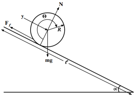
Rolling constraint gives
\[y - R \theta = 0 \nonumber\]
\[x-R=0\nonumber\]
a) Newton’s laws of motion
\[\left( m+\frac{I}{R^{2}}\right) \ddot{y}-mg\sin \alpha =0\nonumber\]
The moment of inertia of a uniform solid circular disk is \(I=\frac{1 }{2}mR^{2}\)
\[F_{f}=\frac{mg}{3}\sin \alpha\nonumber\]
which is smaller than the gravitational force along the plane which is \(mg\sin \alpha .\)
b) Lagrange equations with a minimal set of generalized coordinates
\[mg\sin \alpha =\left( m+\frac{I}{R^{2}}\right) \overset{..}{y}\nonumber\]
Again if \(I=\frac{1}{2}mR^{2}\) then \[\ddot{y}=\frac{2}{3}g\sin \alpha\nonumber\]
The solution for the \(x\) coordinate is trivial. This answer is identical to that obtained using Newton’s laws of motion. Note that no forces have been determined using the single generalized coordinate.
c) Lagrange equation with Lagrange multipliers
\[m\ddot{y}=mg\sin \alpha +\lambda _{1}=\frac{2}{3}mg\sin \alpha\nonumber\]
and the torque is \[-\lambda _{1}R=F_{f}R=I\ddot{\theta}\nonumber\]
d) Lagrange equation using a generalized force
\[\begin{aligned} Q_{y} &=&-F_{f} \\ Q_{\theta } &=&F_{f}R\end{aligned} \]
The Euler-Lagrange equations are:
\[F_{f}=-\frac{mg}{3}\sin \alpha\nonumber\]
The four methods for handling the equations of constraint all are equivalent and result in the same equations of motion. The scalar Lagrangian mechanics is able to calculate the vector forces acting in a direct and simple way. The Newton’s law approach is more intuitive for this simple case and the ease and power of the Lagrangian approach is not apparent for this simple system.
The following series of examples will gradually increase in complexity, and will illustrate the power, elegance, plus superiority of the Lagrangian approach compared with the Newtonian approach.
Example \(\PageIndex{2}\): Two connected masses on frictionless inclined planes
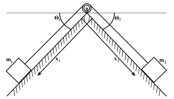
\[T= \frac{1}{2}m_{1}\dot{x}_{1}^{2}+\frac{1}{2}m_{2}\dot{x}_{2}^{2}=\frac{1}{2} \left( m_{1}+m_{2}\right) \dot{x}_{1}^{2}\nonumber\]
The Lagrangian then gives that
\[L=\frac{1}{2}\left( m_{1}+m_{2}\right) \dot{x}_{1}^{2}+m_{1}gx_{1}\sin \theta _{1}+m_{2}g\left( l-x_{1}\right) \sin \theta _{2}\nonumber\]
Therefore \[\begin{aligned} \frac{\partial L}{\partial \dot{x}_{1}} &=&\left( m_{1}+m_{2}\right) \dot{x} _{1} \\ \frac{\partial L}{\partial x_{1}} &=&g\left( m_{1}\sin \theta _{1}-m_{2}\sin \theta _{2}\right)\end{aligned} \]
\[\Lambda _{x_{1}}L=\frac{d}{dt}\frac{\partial L}{\partial \dot{x}_{1}}-\frac{ \partial L}{\partial x_{1}}=0=\left( m_{1}+m_{2}\right) \ddot{x}_{1}-g\left( m_{1}\sin \theta _{1}-m_{2}\sin \theta _{2}\right)\nonumber\]
Note that the system acts as though the inertial mass is \((m_{1}+m_{2})\) while the driving force comes from the difference of the forces. The acceleration is zero if
\[m_{1}\sin \theta _{1}=m_{2}\sin \theta _{2}\nonumber\]
\[\left( m_{1}+m_{2}\right) \ddot{x}_{1}=g\left( m_{1}-m_{2}\right)\nonumber\]
Note that this problem has been solved without any reference to the force in the rope or the normal constraint forces on the inclined planes.
Example \(\PageIndex{3}\): Block sliding on a movable frictionless inclined plane
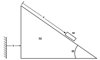
The Lagrangian is \[L=\frac{1}{2} M \dot{x}^{2}+\frac{1}{2} m\left[\dot{x}^{2}+\dot{x}^{\prime 2}+2 \dot{x} \dot{x}^{\prime} \cos \theta\right]+m g x^{\prime} \sin \theta\nonumber\]
Consider the Lagrange-Euler equation for the \(x\) coordinate, \(\Lambda_x L = 0\) which gives
\[\frac{d}{dt}[m(\dot{x}+\dot{x}^{\prime }\cos \theta )+M\dot{x}]=0 \tag{$a$} \label{a2}\]
which states that \([m(\dot{x}+\dot{x}^{\prime }\cos \theta )+M\dot{x }]\) is a constant of motion. This constant of motion is just the total linear momentum of the complete system in the \(x\) direction. That is, conservation of the linear momentum is satisfied automatically by the Lagrangian approach. The Newtonian approach also predicts conservation of the linear momentum since there are no external horizontal forces,
Consider the Lagrange-Euler equation for the \(x^{\prime}\) coordinate, \(\Lambda_{x^{\prime}} L = 0\) which gives
\[\ddot{x}^{\prime }=\frac{g\sin \theta }{1-m\cos ^{2}\theta /(m+M)}\nonumber\]
This example illustrates the flexibility of being able to use non-orthogonal displacement vectors to specify the scalar Lagrangian energy. Newtonian mechanics would require more thought to solve this problem.
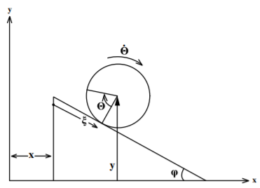
Example \(\PageIndex{4}\): Sphere rolling without slipping down an inclined plane on a frictionless floor
\[\begin{aligned} v_{x} &=& \dot{x}+R\dot{\theta}\cos \varphi \\ v_{y} &=&-R\dot{\theta}\sin \varphi\end{aligned} \]
Assume initial conditions are \(t=0,\xi =0,x=0,\theta =0,y=h,\dot{x}= \dot{\theta}=0.\) Choose the independent coordinates \(x\) and \(\theta\) as generalized coordinates plus the holonomic constraint \(\xi =R\theta\). Then the Lagrangian is \[L=\frac{M}{2}\dot{x}^{2}+\frac{m}{2}\left[ \dot{x}^{2}+r^{2}\dot{\theta} ^{2}+2r\dot{x}\dot{\theta}\cos \varphi \right] +\frac{m}{5}r^{2}\dot{\theta} ^{2}-mg\left( h-r\theta \sin \varphi \right)\nonumber\]
\[x=-\frac{mr\cos \varphi }{M+m}\theta =\frac{5m\sin \left( 2\varphi \right) }{ 4\left[ 7\left( M+m\right) -5m\cos ^{2}\varphi \right] }gt^{2}\nonumber\]
Note that these equations predict conservation of linear momentum for the block plus sphere.
Example \(\PageIndex{5}\): Mass sliding on a rotating straight frictionless rod.
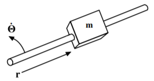
\[\Lambda _{\theta }L=\frac{d}{dt}\frac{\partial L}{\partial \dot{\theta}}- \frac{\partial L}{\partial \theta }=\frac{d}{dt}(mr^{2}\dot{\theta})=0\nonumber\]
Thus the angular momentum is constant \[mr^{2}\dot{\theta}=\text{constant}=p_{\theta }\nonumber\]
The Lagrange equation for \(r\) gives \[\Lambda _{r}L=\frac{d}{dt}\frac{\partial L}{\partial \dot{r}}-\frac{\partial L}{\partial r}=m\ddot{r}-mr\dot{\theta}^{2}=0\nonumber\]
The \(\theta\) equation states that the angular momentum is conserved for this case which is what we expect since there are no external torques acting on the system. The \(r\) equation states that the centrifugal acceleration is \(\ddot{r}=r\omega ^{2}.\) These equations of motion were derived without reference to the forces between the rod and mass.
Example \(\PageIndex{6}\): Spherical pendulum
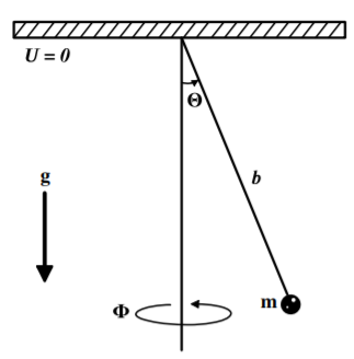
\[U=-mgb\cos \theta\nonumber\]
giving that \[L=\frac{1}{2}mb^{2}\dot{\theta}^{2}+\frac{1}{2}mb^{2}\sin ^{2}\theta \dot{ \phi}^{2}+mgb\cos \theta\nonumber\]
\[mb^{2}\sin ^{2}\theta \dot{\phi}=p_{\phi }=\text{ constant}\nonumber\]
This is just the angular momentum \(p_{\phi }\) for the pendulum rotating in the \(\phi\) direction. Automatically the Lagrange approach shows that the angular momentum \(p_{\phi }\) is a conserved quantity. This is what is expected from Newton’s Laws of Motion since there are no external torques applied about this vertical axis.
The equation of motion for \(\theta\) can be simplified to \[\ddot{\theta}+\frac{g}{b}\sin \theta -\frac{p_{\phi }^{2}\cos \theta }{ m^{2}b^{4}\sin ^{3}\theta }=0\nonumber\]
There are many possible solutions depending on the initial conditions. The pendulum can just oscillate in the \(\theta\) direction, or rotate in the \(\phi\) direction or some combination of these. Note that if \(p_{\phi }\) is zero, then the equation reduces to the simple harmonic pendulum, while the other extreme is when \(\ddot{\theta}=0\) for which the motion is that of a conical pendulum that rotates at a constant angle \(\theta _{0}\) to the vertical axis.
Example \(\PageIndex{7}\): Mass constrained to move on the inside of a frictionless paraboloid
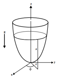
\[x^{2}+y^{2}=\rho ^{2}=az\nonumber\]
with a gravitational potential energy of \(U=mgz.\)
This system is holonomic, scleronomic, and conservative. Choose cylindrical coordinates \(\rho ,\phi ,z\) with respect to the vertical axis of the paraboloid to be the generalized coordinates.
\[g(\rho ,z)=\rho ^{2}-az=0\nonumber\]
The Lagrange multiplier approach will be used to determine the forces of constraint.
For \(\Lambda _{\rho }L=\lambda \frac{\partial g}{\partial \rho }\)
\[\begin{align} \frac{d}{dt}\frac{\partial L}{\partial \dot{r}}-\frac{\partial L}{\partial r} &=&\lambda _{1}2\rho \tag{a} \label{a3} \\ m\left( \ddot{\rho}-\rho \dot{\phi}^{2}\right) &=&\lambda _{1}2\rho \notag\end{align}\]
For \(\Lambda _{\phi }L=\lambda \frac{\partial g}{\partial \phi }\)
\[\frac{d}{dt}\left( m\rho ^{2}\dot{\phi}\right) =\dot{p}_{\phi }=0 \tag{b} \label{b3}\]
Thus the angular momentum \(p_{\phi }\) is conserved, that is, it is a constant of motion.
\[2\rho \dot{\rho}-a\dot{z}=0 \tag{d} \label{d3}\]
The above four equations of motion can be used to determine \(r,\phi .z,\lambda _{1}.\)
\[F_{c}=\lambda _{1}\frac{\partial g(\rho ,z)}{\partial \rho }=-\frac{mg}{a} 2\rho\nonumber\]
Assuming that \(\ddot{\rho}=0,\) then equation \ref{a3} for \(\dot{\phi}=\omega\) and \(\rho =\rho _{0}\) gives
\[F_{c}=-m\rho _{0}\omega ^{2}\nonumber\]
which is the usual centripetal force. These relations also give that the initial angular velocity required for such a stable trajectory with height \(h\) is \[{\small \ }\dot{\phi}=\omega =\sqrt{\frac{2g}{a}}\nonumber\]
Example \(\PageIndex{8}\): Mass on a frictionless plane connected to a plane pendulum
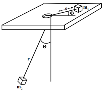
Two masses \(m_{1}\) and \(m_{2}\) are connected by a string of length \(l\). Mass \(m_{1}\) is on a horizontal frictionless table and it is assumed that mass \(m_{2}\) moves in a vertical plane. This is another problem involving holonomic constrained motion. The constraints are:
1) \(m_{1}\) moves in the horizontal plane
2) \(m_{2}\) moves in the vertical plane
3) \(r+s=l.\) Therefore \(\dot{r}=-\dot{s}\)
Thus the Lagrange equations are
\[\begin{aligned} & \Lambda_{r} L=\left(m_{1}+m_{2}\right) \ddot{r}+m_{1}(l-r) \dot{\phi}^{2}-m_{2} r \dot{\theta}^{2}-m_{2} g \cos \theta=0 \\ &
\Lambda_{\theta} L=\frac{d}{d t}\left[m_{2} r^{2} \dot{\theta}\right]+m_{2} g r \sin \theta=0 \end{aligned} \]
that is
\[2 m_{2} \dot{r} \dot{\theta}+r^{2} m_{2} \ddot{\theta}+m_{2} g r \sin \theta=0 \nonumber\]
\[\Lambda _{\phi }L=\frac{d}{dt}\left[ m_{1}\left( l-r\right) ^{2}\dot{\phi} \right] =0\nonumber\]
This last equation is a statement of the conservation of angular momentum. These three differential equations of motion can be solved for known initial conditions.
Example \(\PageIndex{9}\): Two connected masses constrained to slide along a moving rod
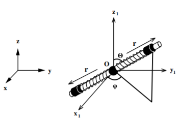
Consider two identical masses \(m,\) constrained to move along the axis of a thin straight rod, of mass \(M\) and length \(l,\) which is free to both translate and rotate. Two identical springs link the two masses to the central point of the rod. Consider only motions of the system for which the extended lengths of the two springs are equal and opposite such that the two masses always are equal distances from the center of the rod keeping the center of mass at the center of the rod. Find the equations of motion for this system.
Use a fixed cartesian coordinate system \((x,y,z)\) and a moving frame with the origin \(O\) at the center of the rod with its cartesian coordinates \((x_{1},y_{1},z_{1})\) being parallel to the fixed coordinate frame as shown in the figure. Let \((r,\theta ,\varphi )\) be the spherical coordinates of a point referring to the center of the moving \((x_{1},y_{1},z_{1})\) frame as shown in the figure. Then the two masses \(m\) have spherical coordinates \((r,\theta ,\varphi )\) and \((-r,\theta ,\varphi )\) in the moving-rod fixed frame. The frictionless constraints are holonomic.
\[L=\frac{1}{2}(M+2m)(\dot{x}^{2}+\dot{y}^{2}+\dot{z}^{2})+m(\dot{r}^{2}+r^{2} \dot{\theta}^{2}+r^{2}\dot{\varphi}^{2}\sin ^{2}\theta )+\frac{1}{24}ML^{2}( \dot{\theta}^{2}+\dot{\varphi}^{2}\sin ^{2}\theta )-K(r-r_{0})^{2}\nonumber\]
Using Lagrange’s equations \(\Lambda _{q_{i}}L=0\) for the generalized coordinates gives.
\[\begin{align} (M+2m)\dot{x} &=&\text{constant} \tag{$\Lambda _{x}L=0$} \\ (M+2m)\dot{y} &=&\text{constant} \tag{$\Lambda _{y}L=0$} \\ (M+2m)\dot{z} &=&\text{constant} \tag{$\Lambda _{z}L=0$} \\ \left( 2mr^{2}+\frac{1}{12}Ml^{2}\right) \dot{\varphi}\sin ^{2}\theta &=& \text{constant} \tag{$\Lambda _{\varphi }L=0$} \\ \ddot{r}-r\dot{\theta}^{2}-r\dot{\varphi}^{2}\sin ^{2}\theta +\frac{K}{m} (r-r_{0}) &=&0 \tag{$\Lambda _{r}L=0$} \\ \left( r^{2}+\frac{Ml^{2}}{24m}\right) \ddot{\theta}+2r\dot{r}\dot{\theta} -\left( r^{2}+\frac{ml^{2}}{24m}\right) \dot{\varphi}^{2}\sin \theta \cos \theta &=&0 \tag{$\Lambda _{\theta }L=0$}\end{align}\]
The first three equations show that the three components of the linear momentum of the center of mass are constants of motion. The fourth equation shows that the component of the angular momentum about the \(z^{\prime }\) axis is a constant of motion. Since the \(z_{1}\) axis has been arbitrarily chosen then the total angular momentum must be conserved. The fifth and sixth equations give the radial and angular equations of motion of the oscillating masses \(m\).