8.5: Applications of Hamiltonian Dynamics

The equations of motion of a system can be derived using the Hamiltonian coupled with Hamilton’s equations of motion, that is, equations \((8.3.11-8.3.13)\).

Formally the Hamiltonian is constructed from the Lagrangian. That is

1. Select a set of independent generalized coordinates \(q_{i}\)
2. Partition the active forces.
3. Construct the Lagrangian \(L(q_{i}, \dot{q}_{i},t)\)
4. Derive the conjugate generalized momenta via \(p_{i}=\frac{\partial L}{ \partial \dot{q}_{i}}\)
5. Knowing \(L,\dot{q}_{i},p_{i}\) derive \(H=\sum_{i}p_{i}\dot{q}_{i}-L\)
6. Derive \(\dot{q}_{k}=\frac{\partial H}{\partial p_{k}}\) and \(\dot{p}_{j}=- \frac{\partial H(\mathbf{q,p,}t\mathbf{)}}{\partial q_{j}} +\sum_{k=1}^{m}\lambda _{k}\frac{\partial g_{k}}{\partial q_{j}} +Q_{j}^{EXC}.\)

This procedure appears to be unnecessarily complicated compared to just using the Lagrangian plus Lagrangian mechanics to derive the equations of motion. Fortunately the above lengthy procedure often can be bypassed for conservative systems. That is, if the following conditions are satisfied;

1. \(L=T(\overset{.}{q})-U(q)\), that is, \(U\left( q\right)\) is independent of the velocity \(\dot{q}\).
2. the generalized coordinates are time independent.

then it is possible to use the fact that

\[H=T+U=E.\nonumber\]

The following five examples illustrate the use of Hamiltonian mechanics to derive the equations of motion.

Example \(\PageIndex{1}\): Motion in a uniform gravitational field

Consider a mass \(m\) in a uniform gravitational field acting in the \(-\mathbf{z}\) direction. The Lagrangian for this simple case is

\[L= \frac{1}{2}m\left( \dot{x}^{2}+\dot{y}^{2}+\dot{z}^{2}\right) -mgz\nonumber\]

Therefore the generalized momenta are \(p_{x}=\frac{\partial L}{ \partial \dot{x}}=m\dot{x},\) \(p_{y}=\frac{\partial L}{\partial \dot{y}}=m \dot{y},\) \(p_{z}=\frac{\partial L}{\partial \dot{z}}=m\dot{z}\). The corresponding Hamiltonian \(H\) is

\[\begin{aligned} H &=&\sum_{i}p_{i}\dot{q}_{i}-L=p_{x}\dot{x}+p_{y}\dot{y}+p_{z}\dot{z}-L \\ &=&\frac{p_{x}^{2}}{m}+\frac{p_{y}^{2}}{m}+\frac{p_{z}^{2}}{m}-\frac{1}{2} \left( \frac{p_{x}^{2}}{m}+\frac{p_{y}^{2}}{m}+\frac{p_{z}^{2}}{m}\right) +mgz=\frac{1}{2}\left( \frac{p_{x}^{2}}{m}+\frac{p_{y}^{2}}{m}+\frac{ p_{z}^{2}}{m}\right) +mgz\end{aligned}\]

Note that the Lagrangian is not explicitly time dependent, thus the Hamiltonian is a constant of motion.

Hamilton’s equations give that \[\begin{aligned} \dot{x} &=&\frac{\partial H}{\partial p_{x}}=\frac{p_{x}}{m}\hspace{1in}- \dot{p}_{x}=\frac{\partial H}{\partial x}=0 \\ \dot{y} &=&\frac{\partial H}{\partial p_{y}}=\frac{p_{y}}{m}\hspace{1in}- \dot{p}_{y}=\frac{\partial H}{\partial y}=0 \\ \dot{z} &=&\frac{\partial H}{\partial p_{z}}=\frac{p_{z}}{m}\hspace{1in}- \dot{p}_{z}=\frac{\partial H}{\partial z}=mg\end{aligned}\]

Combining these gives that \(\ddot{x}=0,\) \(\ddot{y}=0, \ddot{z}=-g\). Note that the linear momenta \(p_{x}\) and \(p_{y}\) are constants of motion whereas the rate of change of \(p_{z}\) is given by the gravitational force \(mg\). Note also that \(H=T+U\) for this conservative system.

Example \(\PageIndex{2}\): One-dimensional harmonic oscillator

Consider a mass \(m\) subject to a linear restoring force with spring constant \(k.\) The Lagrangian \(L=T-U\) equals

\[L=\frac{1}{2}m\dot{x}^{2}-\frac{1}{2}kx^{2}\nonumber\]

Therefore the generalized momentum is

\[p_{x}=\frac{\partial L}{\partial \dot{x}}=m\dot{x}\nonumber\]

The Hamiltonian \(H\) is

\[\begin{aligned} H &=\sum_{i}p_{i}\dot{q}_{i}-L=p_{x}\dot{x}-L \\ &=\frac{p_{x}p_{x}}{m}-\frac{1}{2}\frac{p_{x}^{2}}{m}+\frac{1}{2}kx^{2}= \frac{1}{2}\frac{p_{x}^{2}}{m}+\frac{1}{2}kx^{2}\end{aligned}\]

Note that the Lagrangian is not explicitly time dependent, thus the Hamiltonian will be a constant of motion. Hamilton’s equations give that

\[\dot{x}=\frac{\partial H}{\partial p_{x}}=\frac{p_{x}}{m}\nonumber\]

or

\[p_{x}=m\dot{x}\nonumber\]

In addition

\[-\dot{p}_{x}=\frac{\partial H}{\partial x}=\frac{\partial U}{\partial x}=kx\nonumber\]

Combining these gives that

\[\ddot{x}+\frac{k}{m}x=0\nonumber\]

which is the equation of motion for the harmonic oscillator.

Example \(\PageIndex{3}\): Plane pendulum

The plane pendulum, in a uniform gravitational field \(g,\) is an interesting system to consider. There is only one generalized coordinate, \(\theta\) and the Lagrangian for this system is

\[L= \frac{1}{2}ml^{2}\dot{\theta}^{2}+mgl\cos \theta\nonumber\]

The momentum conjugate to \(\theta\) is

\[p_{\theta }=\frac{\partial L}{\partial \dot{\theta}}=ml^{2}\dot{\theta}\nonumber\] which is the angular momentum about the pivot point.

The Hamiltonian is

\[H=\sum_{i}p_{i}\dot{q}_{i}-L=p_{\theta }\dot{\theta}-L=\frac{1}{2}ml^{2}\dot{ \theta}^{2}-mgl\cos \theta =\frac{p_{\theta }^{2}}{2ml^{2}}-mgl\cos \theta\nonumber\] Hamilton’s equations of motion give

\[\dot{\theta}=\frac{\partial H}{\partial p_{\theta }}=\frac{p_{\theta }}{ ml^{2}}\nonumber\]

\[\overset{.}{\dot{p}_{\theta }=-\frac{\partial H}{\partial \theta }=}-mgl\sin \theta\nonumber\]

Note that the Lagrangian and Hamiltonian are not explicit functions of time, therefore they are conserved. Also the potential is velocity independent and there is no coordinate transformation, thus the Hamiltonian equals the total energy, that is

\[H=\frac{p_{\theta }^{2}}{2ml^{2}}-mgl\cos \theta =E\nonumber\]

where \(E\) is a constant of motion. Note that the angular momentum \(p_{\theta }\) is not a constant of motion since \(\dot{p} _{\theta }\) explicitly depends on \(\theta\).

Figure \(\PageIndex{1}\): Phase-space diagrams for the plane pendulum. The separatrix (bold line) separates the oscillatory solutions from the rolling solutions. The upper (a) shows one complete cycle while the lower (b) shows two complete cycles.

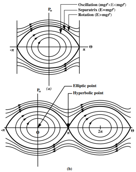
The solutions for the plane pendulum on a \(\left( \theta ,p_{\theta }\right)\) phase diagram, shown in the adjacent figure, illustrate the motion. The upper phase-space plot shows the range \(\left( \theta =\pm \pi ,p_{\theta }\right)\). Note that the \(\theta =+\pi\) and \(-\pi\) correspond to the same physical point, that is the phase diagram should be rolled into a cylinder connected along the dashed lines. The lower phase space plot shows two cycles for \(\theta\) to better illustrate the cyclic nature of the phase diagram. The corresponding state-space diagram is shown in Figure \(3.4.2\). The trajectories are ellipses for low energy \(-mgl<E\,<mgl\) corresponding to oscillations of the pendulum about \(\theta =0\). The center of the ellipse \(\left( 0,0\right)\) is a stable equilibrium point for the oscillation. However, there is a phase change to rotational motion about the horizontal axis when \(\left\vert E\right\vert >mgl\), that is, the pendulum swings around a circle continuously, i.e. it rotates continuously in one direction about the horizontal axis. The phase change occurs at \(E=mgl.\) and is designated by the separatrix trajectory.

The plot of \(p_{\theta }\) versus \(\theta\) for the plane pendulum is better presented on a cylindrical phase space representation since \(\theta\) is a cyclic variable that cycles around the cylinder, whereas \(p_{\theta }\) oscillates equally about zero having both positive and negative values. When wrapped around a cylinder then the unstable and stable equilibrium points will be at diametrically opposite locations on the surface of the cylinder at \(p_{\theta }=0\). For small oscillations about equilibrium, also called librations, the correlation between \(p_{\theta }\) and \(\theta\) is given by the clockwise closed ellipses wrapped on the cylindrical surface, whereas for energies \(\left\vert E\right\vert >mgl\) the positive \(p_{\theta }\) corresponds to counterclockwise rotations while the negative \(p_{\theta }\) corresponds to clockwise rotations.

Example \(\PageIndex{4}\): Hooke's law force constrained to the surface of a cylinder

Figure \(\PageIndex{2}\): Mass attracted to origin by force proportional to distance from origin with the motion constrained to the surface of a cylinder.

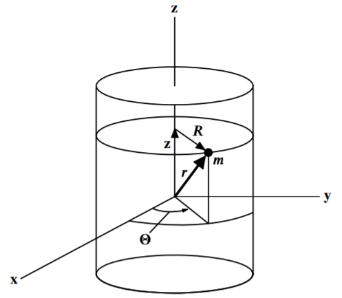
Consider the case where a mass \(m\) is attracted by a force directed toward the origin and proportional to the distance from the origin. Determine the Hamiltonian if the mass is constrained to move on the surface of a cylinder defined by

\[x^{2}+y^{2}=R^{2}\nonumber\]

It is natural to transform this problem to cylindrical coordinates \(\rho ,z,\theta\). Since the force is just Hooke’s law

\[\mathbf{F}=-k\mathbf{r}\nonumber\]

the potential is the same as for the harmonic oscillator, that is

\[U= \frac{1}{2}kr^{2}=\frac{1}{2}k(\rho ^{2}+z^{2})\nonumber\]

This is independent of \(\theta ,\) and thus \(\theta\) is cyclic.

\[p_{z}=\frac{\partial L}{\partial \dot{z}}=m\dot{z} \tag{b} \label{b}\]

The system is conservative, and the transformation from rectangular to cylindrical coordinates does not depend explicitly on time. Therefore the Hamiltonian is conserved and equals the total energy. That is

\[H=\sum_{i}p_{i}\dot{q}_{i}-L=\frac{p_{\theta }^{2}}{2mR^{2}}+\frac{p_{z}^{2} }{2m}+\frac{1}{2}k(R^{2}+z^{2})=E\nonumber\]

The equations of motion then are given by the canonical equations \[\begin{align} \dot{p}_{\theta } &=&-\frac{\partial H}{\partial \theta }=0\hspace{1in}\dot{ \theta}=\frac{\partial H}{\partial p_{\theta }}=\frac{p_{\theta }}{mR^{2}} \tag{c} \label{c} \\ \dot{p}_{z} &=&-\frac{\partial H}{\partial z}=-kz\mathit{\hspace{0.8in}}\dot{ z}=\frac{\partial H}{\partial p_{z}}=\frac{p_{z}}{m} \tag{d} \label{d}\end{align}\]

Equation \ref{a} and \ref{c} imply that

\[p_{\theta }=\frac{\partial L}{\partial \overset{.}{\theta }}=mR^{2}\dot{ \theta}=\text{constant}\nonumber\]

Thus the angular momentum about the axis of the cylinder is conserved, that is, it is a cyclic variable.

Combining equations \ref{b} and \ref{d} implies that

\[\ddot{z}+\frac{k}{m}z=0\nonumber\]

This is the equation for simple harmonic motion with angular frequency \(\omega =\sqrt{\frac{k}{m}}\). The symmetries imply that this problem has the same solutions for the \(z\) coordinate as the harmonic oscillator, while the \(\theta\) coordinate moves with constant angular velocity.

Example \(\PageIndex{5}\): Electron motion in a cylindrical magnetron

A magnetron comprises a hot cylindrical wire cathode that emits electrons and is at a high negative voltage. It is surrounded by a larger diameter concentric cylindrical anode at ground potential. A uniform magnetic field runs parallel to the cylindrical axis of the magnetron. The electron beam excites a multiple set of microwave cavities located around the circumference of the cylindrical wall of the anode. The magnetron was invented in England during World War 2 to generate microwaves required for the development of radar.

Consider a non-relativistic electron of mass \(m\) and charge \(-e\) in a cylindrical magnetron moving between the central cathode wire, of radius \(a\) at a negative electric potential \(-\phi _{0}\), and a concentric cylindrical anode conductor of radius \(R\) which has zero electric potential. There is a uniform constant magnetic field \(B\) parallel to the cylindrical axis of the magnetron.

Using SI units and cylindrical coordinates \((r,\theta ,z)\) aligned with the axis of the magnetron, the electromagnetic force Lagrangian, given in chapter \(6.10,\) equals

\[L= \frac{1}{2}m\mathbf{\dot{r}}^{2}+e(\phi -\mathbf{\dot{r}}\cdot \mathbf{A})\nonumber\]

The electric and vector potentials for the magnetron geometry are

\[\begin{aligned} \phi &=&-\phi _{0}\frac{\ln (\frac{r}{R})}{\ln (\frac{a}{R})} \\ \mathbf{A} &=&\frac{1}{2}Br\hat{e}_{\theta }\end{aligned}\]

Thus expressed in cylindrical coordinates the Lagrangian equals \[L=\frac{1}{2}m\left( \dot{r}^{2}+r^{2}\dot{\theta}^{2}+\dot{z}^{2}\right) +e\phi -\frac{1}{2}eBr^{2}\dot{\theta}\nonumber\]

The generalized momenta are

\[\begin{aligned} p_{r} &=&\frac{\partial L}{\partial \dot{r}}=m\dot{r} \\ p_{\theta } &=&\frac{\partial L}{\partial \dot{\theta}}=mr^{2}\dot{\theta}- \frac{1}{2}eBr^{2} \\ p_{z} &=&\frac{\partial L}{\partial \dot{z}}=m\dot{z}\end{aligned}\]

Note that the vector potential \(A\) contributes an additional term to the angular momentum \(p_{\theta }\).

Using the above generalized momenta leads to the Hamiltonian \[\begin{aligned} H &=&p_{r}\dot{r}+p_{\theta }\dot{\theta}+p_{z}\dot{z}-L \\ &=&\frac{1}{2}m\left( \dot{r}^{2}+r^{2}\dot{\theta}^{2}+\dot{z}^{2}\right) -e\phi +\frac{1}{2}eBr^{2}\dot{\theta} \\ &=&\frac{p_{r}^{2}}{2m}+\frac{1}{2mr^{2}}\left( p_{\theta }+\frac{1}{2} eBr^{2}\right) ^{2}+\frac{p_{z}^{2}}{2m}-e\phi \\ &=&\frac{1}{2m}\left[ p_{r}^{2}+\left( \frac{p_{\theta }}{r}+\frac{1}{2} eBr\right) ^{2}+p_{z}^{2}\right] -e\phi\end{aligned}\]

Note that the Hamiltonian is not an explicit function of time, therefore it is a constant of motion which equals the total energy. \[H=\frac{1}{2m}\left[ p_{r}^{2}+\left( \frac{p_{\theta }}{r}+\frac{1}{2} eBr\right) ^{2}+p_{z}^{2}\right] -e\phi =E\nonumber\]

Since \(\dot{p}_{i}=-\frac{\partial H}{\partial q_{i}},\) and if \(H\) is not an explicit function of \(q_{i},\) then \(\dot{p}_{i}=0,\) that is, \(p_{i}\) is a constant of motion. Thus \(p_{\theta }\) and \(p_{z}\) are constants of motion.

Consider the initial conditions \(r=a,\dot{r}=\dot{\theta}=\dot{z}=0\). Then \[\begin{aligned} p_{\theta } &=&\frac{\partial L}{\partial \dot{\theta}}=mr^{2}\dot{\theta}- \frac{1}{2}eBr^{2}=-\frac{1}{2}eBa^{2} \\ p_{z} &=&0 \\ H &=&\frac{1}{2m}\left[ p_{r}^{2}+\left( \frac{p_{\theta }}{r}+\frac{1}{2} eBr\right) ^{2}+p_{z}^{2}\right] +e\phi _{0}\frac{\ln (\frac{r}{R})}{\ln ( \frac{a}{R})}=e\phi _{0}\end{aligned}\]

Note that at \(r=R,\) then \(p_{r}\) is given by the last equation since the Hamiltonian equals a constant \(e\phi _{0}\). That is, assuming that \(a<<R\) then

\[p_{r}^{2}=2me\phi _{0}-(\frac{1}{2}eBR)^{2}\nonumber\]

Define a critical magnetic field by

\[B_{c}\equiv \frac{2}{R}\sqrt{\frac{2m\phi _{0}}{e}}\nonumber\]

then

\[\left( p_{r}^{2}\right) _{r=R}=\left( B_{c}^{2}-B^{2}\right) (\frac{1}{2} eR)^{2}\nonumber\]

Note that if \(B<B_{c}\) then \(p_{r}\) is real at \(r=R\). However, if \(B>B_{c}\) then \(p_{r}\) is imaginary at \(r=R\) implying that there must be a maximum orbit radius \(r_{0}\) for the electron where \(r_{0}<R\). That is, the electron trajectories are confined spatially to coaxial cylindrical orbits concentric with the magnetron electromagnetic fields. These closed electron trajectories excite the microwave cavities located in the nearby outer cylindrical wall of the anode.