12.9: Routhian Reduction for Rotating Systems

The Routhian reduction technique, that was introduced in chapter \(8.6\), is a hybrid variational approach. It was devised by Routh to handle the cyclic and non-cyclic variables separately in order to simultaneously exploit the differing advantages of the Hamiltonian and Lagrangian formulations. The Routhian reduction technique is a powerful method for handling rotating systems ranging from galaxies to molecules, or deformed nuclei, as well as rotating machinery in engineering. A valuable feature of the Hamiltonian formulation is that it allows elimination of cyclic variables which reduces the number of degrees of freedom to be handled. As a consequence, cyclic variables are called ignorable variables in Hamiltonian mechanics. The Lagrangian, the Hamiltonian and the Routhian all are scalars under rotation and thus are invariant to rotation of the frame of reference. Note that often there are only two cyclic variables for a rotating system, that is, \(\dot{\theta} = \boldsymbol{\omega}\) and the corresponding canonical total angular momentum \(p_{\theta} = \mathbf{J}\).

As mentioned in chapter \(8.6\), there are two possible Routhians that are useful for handling rotation frames of reference. For rotating systems the cyclic Routhian \(R_{cyclic}\) simplifies to

\[R_{cyclic}\left(q_{1}, \ldots, q_{n} ; \dot{q}_{1}, \ldots, \dot{q}_{s} ; p_{s+1}, \ldots, p_{n} ; t\right)=H_{cyclic}-L_{noncyclic}=\boldsymbol{\omega} \cdot \mathbf{J}-L \label{12.43}\]

This Routhian behaves like a Hamiltonian for the ignorable cyclic coordinates \(\omega, \mathbf{J}\). Simultaneously it behaves like a negative Lagrangian \(L_{noncyclic}\) for all the other coordinates.

The non-cyclic Routhian \(R_{noncyclic}\) complements \(R_{cyclic}\) in that it is defined as

\[R_{noncyclic}\left(q_{1}, \ldots, q_{n} ; p_{1}, \ldots, p_{s} ; \dot{q}_{s+1}, \ldots, \dot{q}_{n} ; t\right)=H_{noncyclic}-L_{cyclic}=H - \boldsymbol{\omega} \cdot \mathbf{J} \label{12.44}\]

This non-cyclic Routhian behaves like a Hamiltonian for all the non-cyclic variables and behaves like a negative Lagrangian for the two cyclic variables \(\omega , p_{\omega}\). Since the cyclic variables are constants of motion, then \(R_{noncyclic}\) is a constant of motion that equals the energy in the rotating frame if \(H\) is a constant of motion. However, \(R_{noncyclic}\) does not equal the total energy since the coordinate transformation is time dependent, that is, the Routhian \(R_{noncyclic}\) corresponds to the energy of the non-cyclic parts of the motion.

For example, the Routhian \(R_{noncyclic}\) for a system that is being cranked about the \(\phi\) axis at some fixed angular frequency \(\dot{\phi} = \omega\), with corresponding total angular momentum \(\mathbf{p}\phi = \mathbf{J}\), can be written as¹

\[\begin{align} R_{noncyclic} & = & H − \boldsymbol{\omega} \cdot \mathbf{J} \label{12.45} \\ & = & \frac{1}{2} m \left[ \mathbf{V} \cdot \mathbf{V} + \mathbf{v}^{\prime\prime} \cdot \mathbf{v}^{\prime\prime}+2\mathbf{V} \cdot \mathbf{v}^{\prime\prime}+2\mathbf{V} \cdot (\boldsymbol{\omega} \times \mathbf{r}^{\prime} )+2v^{\prime\prime} \cdot (\boldsymbol{\omega} \times \mathbf{r}^{\prime} )+(\boldsymbol{\omega} \times \mathbf{r}^{\prime} )^2 \right] − \boldsymbol{\omega} \cdot \mathbf{J} + U(r) \notag \end{align}\]

Note that \(R_{noncyclic}\) is a constant of motion if \(\frac{\partial L}{\partial t} = 0\), which is the case when the system is being cranked at a constant angular frequency. However the Hamiltonian in the rotating frame \(H_{rot} = H − \boldsymbol{\omega} \cdot \mathbf{J}\) is given by \(R_{noncyclic} = H_{rot} \neq E\) since the coordinate transformation is time dependent. The canonical Hamilton equations for the fourth and fifth terms in the bracket can be identified with the Coriolis force \(2m\boldsymbol{\omega} \times \mathbf{v}^{\prime\prime}\), while the last term in the bracket is identified with the centrifugal force. That is, define

\[U_{cf} \equiv - \frac{1}{2} m (\boldsymbol{\omega} \times \mathbf{r}^{\prime} )^2 \label{12.46}\]

where the gradient of \(U_{cf}\) gives the usual centrifugal force.

\[\mathbf{F}_{c f}=-\nabla U_{c f}=\frac{m}{2} \nabla\left[\omega^{2} r^{\prime 2}-\left(\boldsymbol{\omega} \cdot \mathbf{r}^{\prime}\right)^{2}\right]=m\left[\omega^{2} \mathbf{r}^{\prime}-\left(\boldsymbol{\omega} \cdot \mathbf{r}^{\prime}\right) \boldsymbol{\omega}\right]=-m \boldsymbol{\omega} \times\left(\boldsymbol{\omega} \times \mathbf{r}^{\prime}\right)\label{12.47}\]

The Routhian reduction method is used extensively in science and engineering to describe rotational motion of rigid bodies, molecules, deformed nuclei, and astrophysical objects. The cyclic variables describe the rotation of the frame and thus the Routhian \(R_{noncyclic} = H_{rot}\) corresponds to the Hamiltonian for the non-cyclic variables in the rotating frame.

Example \(\PageIndex{1}\): Cranked plane pendulum

Figure \(\PageIndex{1}\): Cranked plane pendulum that is cranked around the vertical axis with angular velocity \(\dot{\phi} = \omega\).

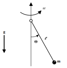
The cranked plane pendulum, which is also called the rotating plane pendulum, comprises a plane pendulum that is cranked around a vertical axis at a constant angular velocity \(\dot{\phi} = \omega\) as determined by some external drive mechanism. The parameters are illustrated in the adjacent figure. The cranked pendulum nicely illustrates the advantages of working in a non-inertial rotating frame for a driven rotating system. Although the cranked plane pendulum looks similar to the spherical pendulum, there is one very important difference; for the spherical pendulum \(p_{\phi} = ml^2 \sin^2 \theta \dot{\phi}\) is a constant of motion and thus the angular velocity varies with \(\theta\), i.e. \(\dot{\phi} = \frac{p_{\phi}}{ml^2 \sin^2 \theta}\), whereas for the cranked plane pendulum, the constant of motion is \(\dot{\phi} = \omega\) and thus the angular momentum varies with \(\theta\), i.e. \(p_{\phi} = l \sin^2 \theta \omega\). For the cranked plane pendulum, the energy must flow into and out of the cranking drive system that is providing the constraint force to satisfy the equation of constraint

\[g_{\phi} = \dot{\phi} − \omega = 0 \notag\]

The easiest way to solve the equations of motion for the cranked plane pendulum is to use generalized coordinates to absorb the equation of constraint and applied constraint torque. This is done by incorporating the \(\dot{\phi} = \omega\) constraint explicitly in the Lagrangian or Hamiltonian and solving for just \(\theta\) in the rotating frame.

Assuming that \(\dot{\phi} = \omega\), and using generalized coordinates to absorb the cranking constraint forces, then the Lagrangian for the cranked pendulum can be written as.

\[L = \frac{1}{2} ml^2 (\dot{\theta}^2 + \sin^2 \theta \omega^2) + mgl \cos \theta \notag\]

The momentum conjugate to \(\theta\) is

\[p_{\theta} = \frac{\partial L}{\partial \dot{\theta}} = ml^2 \dot{\theta} \notag\]

Consider the Routhian \(R_{noncyclic} = p_{\theta} \dot{\theta} − L = H − p_{\phi} \dot{\phi}\) which acts as a Hamiltonian \(H_{rot}\) in the rotating frame

\[R_{noncyclic} = p_{\theta} \dot{\theta} − L = H - p_{\phi} \dot{\phi} = \frac{p^2_{\theta}}{2ml^2} - \frac{1}{2} ml^2 \omega^2 \sin^2 \theta − mgl \cos \theta \nonumber\]

Note that if \(\dot{\phi} = \omega\) is constant, then \(R_{noncyclic}\) is a constant of motion for rotation about the \(\phi\) axis since it is independent of \(\phi\). Also \(\frac{dR_{noncyclic}}{dt} = −\frac{\partial L}{\partial t} = 0\) thus the energy in the rotating non-inertial frame of the pendulum \(R_{noncyclic} = H_{rot} = H − p_{\phi} \dot{\phi}\) is a constant of motion, but it does not equal the total energy since the rotating coordinate transformation is time dependent. The driver that cranks the system at a constant \(\omega\) provides or absorbs the energy \(dW = dE = \omega dp_{\phi}\) as \(\theta\) changes in order to maintain a constant \(\omega\).

The Routhian \(R_{noncyclic}\) can be used to derive the equations of motion using Hamiltonian mechanics.

\[\dot{\theta} = \frac{\partial R_{noncyclic}}{\partial p_{\theta}} = \frac{p_{\theta}}{ml^2} \notag\]

\[\dot{p}_{\theta} = −\frac{\partial R_{noncyclic}}{\partial \theta} = −mgl \sin \theta \left[ 1 − \frac{l}{g} \cos \theta \omega^2 \right] \nonumber\]

Since \(\dot{p}_{\theta} = m;^2 \ddot{\theta}\), then the equation of motion is

\[\ddot{\theta} + \frac{g}{l} \sin \theta \left[ 1 − \frac{l}{g} \cos \theta \omega^2 \right] = 0 \label{alpha} \tag{$\alpha$}\]

Assuming that \(\sin \theta \approx \theta\), then Equation \ref{alpha} leads to linear harmonic oscillator solutions about a minimum at \(\theta = 0\) if the term in brackets is positive. That is, when the bracket \(\left[ 1 − \frac{l}{g} \cos \theta \omega^2 \right] > 0\) then equation \(\ref{alpha}\) corresponds to a harmonic oscillator with angular velocity \(\Omega\) given by

\[\Omega^2 = \frac{g}{l} \sin \theta \left[ 1 − \frac{l}{g} \cos \theta \omega^2 \right] \notag\]

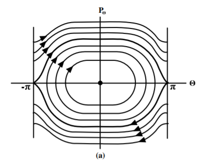
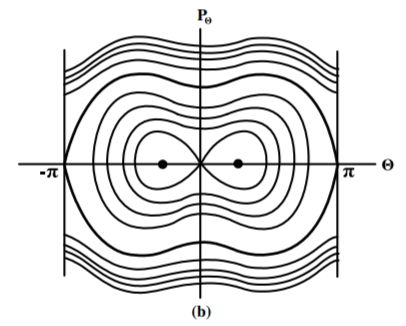
The adjacent figure shows the phase-space diagrams for a plane pendulum rotating about a vertical axis at angular velocity \(\omega\) for (a) \(\omega < \sqrt{\frac{g}{l}}\) and (b) \(\omega > \sqrt{\frac{g}{l}}\). The upper phase plot shows small \(\omega\) when the square bracket of Equation \ref{alpha} is positive and the the phase space trajectories are ellipses around the stable equilibrium point \((0, 0)\). As \(\omega\) increases the bracket becomes smaller and changes sign when \(\omega^2 \cos \theta = \frac{g}{l}\). For larger \(\omega\) the bracket is negative leading to hyperbolic phase space trajectories around the \((\theta , p_{\theta} ) = (0, 0)\) equilibrium point, that is, an unstable equilibrium point. However, new stable equilibrium points now occur at angles \((\theta , p_{\theta} ) =(\pm \theta_0, 0)\) where \(\cos \theta_0 = \frac{g}{l \omega^2}\). That is, the equilibrium point \((0, 0)\) undergoes bifurcation as illustrated in the lower figure. These new equilibrium points are stable as illustrated by the elliptical trajectories around these points. It is interesting that these new equilibrium points \(\pm \theta_0\) move to larger angles given by \(\cos \theta_0 = \frac{g}{l\omega^2}\) beyond the bifurcation point at \(\frac{g}{l\omega^2} = 1\). For low energy the mass oscillates about the minimum at \(\theta = \theta_0\) whereas the motion becomes more complicated for higher energy. The bifurcation corresponds to symmetry breaking since, under spatial reflection, the equilibrium point is unchanged at low rotational frequencies but it transforms from \(+\theta_0\) to \(−\theta_0\) once the solution bifurcates, that is, the symmetry is broken. Also chaos can occur at the separatrix that separates the bifurcation. Note that either the Lagrange multiplier approach, or the generalized force approach, can be used to determine the applied torque required to ensure a constant \(\omega\) for the cranked pendulum.

Figure \(\PageIndex{2}\): Phase-space diagrams for the plane pendulum cranked at angular velocity \(\omega\) about a vertical axis. Figure \(\PageIndex{2a}\) is for \(\omega < \frac{g}{l}\) while \(\PageIndex{2b}\) is for \(\omega > \frac{g}{l}\).

Example \(\PageIndex{2}\): Nucleon orbits in deformed nuclei

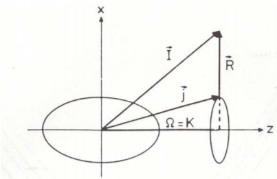
Consider the rotation of axially-symmetric, prolate-deformed nucleus. Many nuclei have a prolate spheroidal shape, (the shape of a rugby ball) and they rotate perpendicular to the symmetry axis. In the non-inertial body-fixed frame, pairs of nucleons, each with angular momentum \(j\), are bound in orbits with the projection of the angular momentum along the symmetry axis being conserved with value \(\Omega = K\), which is a cyclic variable. Since the nucleus is of dimensions \(10^{−14}\) \(m\), quantization is important and the quantized binding energies of the individual nucleons are separated by spacings \(\leq 500\) \(keV\).

Figure \(\PageIndex{3}\): Schematic diagram for the strong coupling of a nucleon to the deformation axis. The projection of \(I\) on the symmetry axis is \(K\), and the projection of \(j\) is \(\Omega\). For axial symmetry Noether’s theroem gives that the projection of the angular momentum \(K\) on the symmetry axis is a conserved quantity.

The Lagrangian and Hamiltonian are scalars and can be evaluated in any coordinate frame of reference. It is most useful to calculate the Hamiltonian for a deformed body in the non-inertial rotating body-fixed frame of reference. The bodyfixed Hamiltonian corresponds to the Routhian \(R_{noncyclic}\)

\[R_{noncyclic} = H − \boldsymbol{\omega} \cdot \mathbf{J}\notag\]

where it is assumed that the deformed nucleus has the symmetry axis along the \(z\) direction and rotates about the \(x\) axis. Since the Routhian is for a non-inertial rotating frame of reference it does not include the total energy but, if the shape is constant in time, then \(R_{noncyclic}\) and the corresponding body-fixed Hamiltonian are conserved and the energy levels for the nucleons bound in the spheroidal potential well can be calculated using a conventional quantum mechanical model.

For a prolate spheroidal deformed potential well, the nucleon orbits that have the angular momentum nearly aligned to the symmetry axis correspond to nucleon trajectories that are restricted to the narrowest part of the spheroid, whereas trajectories with the angular momentum vector close to perpendicular to the symmetry axis have trajectories that probe the largest radii of the spheroid. The Heisenberg Uncertainty Principle, mentioned in chapter \(3.11.3\), describes how orbits restricted to the smallest dimension will have the highest linear momentum, and corresponding kinetic energy, and vise versa for the larger sized orbits. Thus the binding energy of different nucleon trajectories in the spheroidal potential well depends on the angle between the angular momentum vector and the symmetry axis of the spheroid as well as the deformation of the spheroid. A quantal nuclear model Hamiltonian is solved for assumed spheroidal-shaped potential wells. The corresponding orbits each have angular momenta \(\mathbf{j}_i\) for which the projection of the angular momentum along the symmetry axis \(\Omega_i\) is conserved, but the projection of \(\mathbf{j}_i\) in the laboratory frame \(j_z\) is not conserved since the potential well is not spherically symmetric. However, the total Hamiltonian is spherically symmetric in the laboratory frame, which is satisfied by allowing the deformed spheroidal potential well to rotate freely in the laboratory frame, and then \(j^2_i\), \(j_{i,z}\), and \(\Omega_i\) all are conserved quantities. The attractive residual nucleon-nucleon pairing interaction results in pairs of nucleons being bound in time-reversed orbits \((j \times j)^0\), that is, with resultant total spin zero, in this spheroidal nuclear potential. Excitation of an even-even nucleus can break one pair and then the total projection of the angular momentum along the symmetry axis is \(K = |\Omega_1 \pm \Omega_2|\), depending on whether the projections are parallel or antiparallel. More excitation energy can break several pairs and the projections continue to be additive. The binding energies calculated in the spheroidal potential well must be added to the rotational energy \(E_{rot} = \frac{\mathcal{J}}{2} \omega^2\) to get the total energy, where \(\mathcal{J}\) is the moment of inertia. Nuclear structure measurements are in good agreement with the predictions of nuclear structure calculations that employ the Routhian approach.

---

¹For clarity sections \((12.2)\) to \((12.8)\) of this chapter adopted a naming convention that uses unprimed coordinates with the subscript \(fix\) for the inertial frame of reference, primed coordinates with the subscript \(mov\) for the translating coordinates, and double-primed coordinates with the subscript \(rot\) for the translating plus rotating frame. For brevity the subsequent discussion omits the redundant subscripts \(fix\), \(mov\), \(rot\) since the single and double prime superscripts completely define the moving and rotating frames of reference.