14.7: Two-body coupled oscillator systems

The two-body coupled oscillator is the simplest coupled-oscillator system that illustrates the general features of coupled oscillators. The following four examples involve parallel and series couplings of two linear oscillators or two plane pendula.

Example \(\PageIndex{1}\): Two coupled linear oscillators

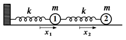
The coupled double-oscillator problem, Figure \(14.2.1\) discussed in chapter \(14.2\), can be used to demonstrate that the general analytic theory gives the same solution as obtained by direct solution of the equations of motion in chapter \(14.2\).

1) The first stage is to determine the potential and kinetic energies using an appropriate set of generalized coordinates, which here are \(x_1\) and \(x_2\). The potential energy is

\[U=\frac{1}{2} \kappa x_{1}^{2}+\frac{1}{2} \kappa x_{2}^{2}+\frac{1}{2} \kappa^{\prime}\left(x_{2} - x_{1}\right)^{2} = \frac{1}{2} \left( \kappa + \kappa^{\prime} \right) x_{1}^{2}+\frac{1}{2} \left( \kappa + \kappa^{\prime} \right) x_{2}^{2}-\kappa^{\prime} x_{1} x_{2} \nonumber\]

while the kinetic energy is given by

\[T = \frac{1}{2}m\dot{x}^2_1 + \frac{1}{2}m\dot{x}^2_2 \nonumber\]

2) The second stage is to evaluate the potential energy \(V\) and kinetic energy \(T\) tensors. The potential energy tensor \(V\) is nondiagonal since \(V_{jk}\) gives

\[V_{11} \equiv \left( \frac{\partial^{2} U}{\partial q_{1} \partial q_{1}} \right)_{0} = \kappa+\kappa^{\prime}=V_{22} \nonumber\]

\[V_{12} =\left( \frac{\partial^{2} U}{\partial q_{1} \partial q_{2}}\right)_{0}=-\kappa^{\prime}=V_{21} \nonumber\]

That is, the potential energy tensor \(V\) is

\[\mathbf{V} \begin{Bmatrix} \kappa + \kappa^{\prime} & -\kappa^{\prime} \\ -\kappa^{\prime} & \kappa + \kappa^{\prime} \end{Bmatrix} \nonumber\]

Similarly, the kinetic energy is given by

\[T = \frac{1}{2}m\dot{x}^2_1 + \frac{1}{2}m\dot{x}^2_2 = \frac{1}{2}\sum_{j,k} T_{jk}\dot{q}_j\dot{q}_k \nonumber\]

Since \(T_{11} = T_{22} = m\) and \(T_{12} = T_{21} = 0\) then the kinetic energy tensor \(T\) is

\[\mathbf{T} \begin{Bmatrix} m & 0 \\ 0 & m \end{Bmatrix} \nonumber\]

Note that for this case, the kinetic energy tensor \(T\) equals the mass tensor, which is diagonal, whereas the potential energy tensor equals the spring constant tensor, which is nondiagonal.

3) The third stage is to use the potential energy \(V\) and kinetic energy \(T\) tensors to evaluate the secular determinant using equations \((14.6.26)\)

\[\begin{vmatrix} \kappa + \kappa^{\prime} - m\omega^2 & -\kappa^{\prime} \\ -\kappa^{\prime} & \kappa + \kappa^{\prime} - m\omega^2 \end{vmatrix} = 0 \nonumber\]

The expansion of this secular determinant yields

\[(\kappa + \kappa^{\prime} - m\omega^2)^2 - \kappa^{\prime 2} = 0 \nonumber\]

That is

\[(\kappa + \kappa^{\prime} - m\omega^2) = \pm\kappa^{\prime} \nonumber\]

Solving for \(\omega_r\) gives

\[\omega_r = \sqrt{\frac{\kappa + \kappa^{\prime} \pm \kappa^{\prime}}{m}} \nonumber\]

The solutions are

\[\omega_1 = \sqrt{\frac{\kappa + 2\kappa^{\prime}}{m}} \nonumber\]

\[\omega_2 = \sqrt{\frac{\kappa}{m}} \nonumber\]

which is the same as derived previously, (equations \((14.2.7-14.2.9)\)).

4) The fourth step is to insert either one of these eigenfrequencies into the secular equation

\[\sum_j (V_{jk} - \omega^2_r T_{jk}) a_{jr} = 0 \nonumber\]

Consider the secular equation \(a\) for \(k = 1\)

\[( \kappa + \kappa^{\prime} − \omega^2_rM) a_{1r} − \kappa^{\prime} a_{2r} = 0 \nonumber\]

Then for the first eigenfrequency \(\omega_1\), that is, \(k = 1\), \(r = 1\)

\[(\kappa + \kappa^{\prime} − \kappa − 2\kappa^{\prime} ) a_{11} − \kappa^{\prime} a_{21} = 0 \nonumber\]

which simplifies to

\[a_{jr} = a_{11} = −a_{21} \nonumber\]

Similarly, for the other eigenfrequency \(\omega_2\), that is, \(k = 1\), \(r = 2\)

\[(\kappa + \kappa^{\prime} − \kappa ) a_{12} − \kappa^{\prime} a_{22} = 0 \nonumber\]

which simplifies to

\[a_{jr} = a_{12} = a_{22} \nonumber\]

5) The final stage is to write the general coordinates in terms of the normal coordinates \(\eta_r (t) \equiv \beta_r e^{i\omega_r t}\). Thus

\[x_1 = a_{11}\eta_1 + a_{12}\eta_2 = a_{11}\eta_1 + a_{22}\eta_2 \nonumber\]

and

\[x_2 = a_{21}\eta_1 + a_{22}\eta_2 = −a_{11}\eta_1 + a_{22}\eta_2 \nonumber\]

Adding or subtracting gives that the normal modes are

\[\eta_1 = \frac{1}{2a_{11}} (x_1 − x_2) \nonumber\]

\[\eta_2 = \frac{1}{2a_{22}} (x_2 + x_1) \nonumber\]

Thus the symmetric normal mode \(\eta_2\) corresponds to an oscillation of the center-of-mass with the lower frequency \(\omega_2 = \sqrt{\frac{\kappa}{m}}\). This frequency is the same as for one single mass on a spring of spring constant \(\kappa\) which is as expected since they vibrate in unison and thus the coupling spring force does not act. The antisymmetric mode \(\eta_1\) has the higher frequency \(\omega_1 = \sqrt{\frac{\kappa + 2\kappa^{\prime}}{m}}\) since the restoring force includes both the main spring plus the coupling spring.

The above example illustrates that the general analytic theory for coupled linear oscillators gives the same answer as obtained in chapter \(14.2\) using Newton’s equations of motion. However, the general analytic theory is a more powerful technique for solving complicated coupled oscillator systems. Thus the general analytic theory will be used for solving all the following coupled oscillator problems.

Example \(\PageIndex{2}\): Two equal masses series-coupled by two equal springs

Figure \(\PageIndex{1}\): Two equal masses series-coupled by two equal springs.

Consider the series-coupled system shown in the figure.

1) The first stage is to determine the potential and kinetic energies using an appropriate set of generalized coordinates, which here are \(x_1\) and \(x_2\). The potential energy is

\[U=\frac{1}{2} \kappa x_{1}^{2} +\frac{1}{2} \kappa \left(x_{2} - x_{1}\right)^{2} = \kappa x_{1}^{2}+\frac{1}{2} \kappa x_{2}^{2}-\kappa x_{1} x_{2} \nonumber\]

while the kinetic energy is given by

\[T = \frac{1}{2}m\dot{x}^2_1 + \frac{1}{2}m\dot{x}^2_2 \nonumber\]

2) The second stage is to evaluate the potential energy \(V\) and mass \(T\) tensors. The potential energy tensor \(V\) is nondiagonal since \(V_{jk}\) gives

\[V_{11} \equiv \left( \frac{\partial^{2} U}{\partial q_{1} \partial q_{1}} \right)_{0} = 2\kappa \nonumber\]

\[V_{12} =\left( \frac{\partial^{2} U}{\partial q_{1} \partial q_{2}}\right)_{0}=-\kappa =V_{21} \nonumber\]

\[V_{22} =\left( \frac{\partial^{2} U}{\partial q_{2} \partial q_{2}}\right)_{0}= \kappa \nonumber\]

That is, the potential energy tensor \(V\) is

\[\mathbf{V} \begin{Bmatrix} 2\kappa & -\kappa \\ -\kappa & \kappa \end{Bmatrix} \nonumber\]

Similarly, since the kinetic energy is given by

\[T = \frac{1}{2}m\dot{x}^2_1 + \frac{1}{2}m\dot{x}^2_2 = \frac{1}{2}\sum_{j,k} m_{jk}\dot{q}_j\dot{q}_k \nonumber\]

then \(T_{11} = T_{22} = m\) and \(T_{12} = T_{21} = 0\). Thus the kinetic energy tensor \(T\) is

\[\mathbf{T} \begin{Bmatrix} m & 0 \\ 0 & m \end{Bmatrix} \nonumber\]

Note that for this case the kinetic energy tensor is diagonal whereas the potential energy tensor is nondiagonal.

3) The third stage is to use the potential energy \(V\) and kinetic energy \(T\) tensors to evaluate the secular determinant using equation \((14.6.26)\)

\[\begin{vmatrix} 2\kappa - m\omega^2 & -\kappa \\ -\kappa & \kappa - m\omega^2 \end{vmatrix} = 0 \nonumber\]

The expansion of this secular determinant yields

\[( 2\kappa − m\omega^2) (\kappa − m\omega^2) − \kappa^2 = 0 \nonumber\]

That is

\[\omega^4 − 3 \frac{\kappa }{m} \omega^2 + \frac{\kappa^2}{m^2} = 0 \nonumber\]

The solutions are

\[\omega_1 = \frac{\sqrt{5}+1}{2}\sqrt{\frac{\kappa}{ m}} \quad \omega_2 = \frac{\sqrt{5}-1}{2} \sqrt{\frac{\kappa}{ m}} \nonumber\]

4) The fourth step is to insert these eigenfrequencies into the secular equation \((14.6.25)\)

\[\sum_j (V_{jk} - \omega^2_r T_{jk}) a_{jr} = 0 \nonumber\]

Consider \(k = 1\) in the above equation

\[( 2\kappa − \omega^2_rM) a_{1r} − \kappa a_{2r} = 0 \nonumber\]

Then for eigenfrequency \(\omega_1\), that is, \(k = 1\), \(r = 1\)

\[\frac{\sqrt{5} − 1}{2} a_{11} = −a_{21} \nonumber\]

Similarly, for \(k = 1\), \(r = 2\)

\[\frac{\sqrt{5} + 1}{2} a_{12} = a_{22} \nonumber\]

5) The final stage is to write the general coordinates in terms of the normal coordinates \(\eta_r (t) \equiv \beta_re^{i\omega_rt}\).

Thus

\[x_1 = a_{11}\eta_1 + a_{12}\eta_2 = a_{11}\eta_1 + \frac{2a_{22}}{ \sqrt{5} +1}\eta_2 \nonumber\]

and

\[x_2 = a_{21}\eta_1 + a_{22}\eta_2 = − \left(\frac{\sqrt{5} − 1}{2} \right) a_{11}\eta_1 + a_{22}\eta_2 \nonumber\]

Adding or subtracting gives that the normal modes are

\[\eta_1 = \frac{1}{a_{11} \sqrt{5}} \left( x_1 − \left(\frac{\sqrt{5} − 1}{ 2} \right) x_2 \right) \nonumber\]

\[\eta_2 = \frac{1}{a_{22} \sqrt{5}} \left( x_1 + \left(\frac{\sqrt{5} +1}{2} \right) x_2 \right) \nonumber\]

Thus the symmetric normal mode has the lower frequency \(\omega_2 = \frac{\sqrt{5} −1}{2} \sqrt{\frac{\kappa}{ m}}\). The antisymmetric mode has the frequency \(\omega_1 = \frac{\sqrt{5} +1}{2}\sqrt{\frac{\kappa}{m}}\) since both springs provide the restoring force. This case is interesting in that for both normal modes, the amplitudes for the motion of the two masses are different.

Example \(\PageIndex{3}\): Two parallel-coupled plane pendula

Figure \(\PageIndex{2}\): Two parallel-coupled plane pendula.

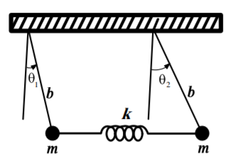
Consider the coupled double pendulum system shown in the adjacent figure, which comprises two parallel plane pendula weakly coupled by a spring. The angles \(\theta_1\) and \(\theta_2\) are chosen to be the generalized coordinates and the potential energy is chosen to be zero at equilibrium. Then the kinetic energy is

\[T = \frac{1}{2} m \left( b\dot{\theta}_1 \right)^2 + \frac{1}{2} m \left( b\dot{\theta}_2 \right)^2 \nonumber\]

As discussed in chapter \(3\), it is necessary to make the small-angle approximation in order to make the equations of motion for the simple pendulum linear and solvable analytically. That is,

\[\begin{aligned} U &=m g b\left(1-\cos \theta_{1}\right)+m g b\left(1-\cos \theta_{2}\right) + \frac{1}{2} \kappa\left(b \sin \theta_{1}-b \sin \theta_{2} \right)^{2} \\ & \simeq \frac{m g b} {2}\left(\theta_{1}^{2} + \theta_{2}^{2} \right) + \frac{\kappa b^{2}}{2}\left(\theta_{1}-\theta_{2}\right)^{2}
\end{aligned} \]

assuming the small angle approximation \(\sin \theta \approx \theta\) and \((1 − \cos \theta_1) = \frac{\theta^2}{2}\).

The second stage is to evaluate the kinetic energy \(T\) and potential energy \(V\) tensors

\[\mathbf{T} = \begin{Bmatrix} mb^2 & 0 \\ 0 & mb^2 \end{Bmatrix} \quad \mathbf{V} = \begin{Bmatrix} mgb + \kappa b^2 & -\kappa b^2 \\ -\kappa b^2 & mgb + \kappa b^2 \end{Bmatrix} \nonumber\]

Note that for this case the kinetic energy tensor is diagonal whereas the potential energy tensor is nondiagonal.

The third stage is to evaluate the secular determinant

\[\begin{vmatrix} mgb + \kappa b^2 - \omega^2mb^2 & -\kappa b^2 \\ -\kappa b^2 & mgb + \kappa b^2 - \omega^2mb^2 \end{vmatrix} = 0 \nonumber\]

which gives the characteristic equation

\[( mgb + \kappa b^2 − \omega^2mb^2)^2 = ( \kappa b^2)^2 \nonumber\]

or

\[mg + \kappa b − \omega^2mb = \pm\kappa b \nonumber\]

The two solutions are

\[\omega^2_1 = \frac{g}{b} \quad \omega^2_2 = \frac{g}{b} + \frac{2\kappa}{ m} \nonumber\]

The fourth step is to insert these eigenfrequencies into equation \((14.6.25)\)

\[\sum_j (V_{jk} - \omega^2_r T_{jk}) a_{jr} = 0 \nonumber\]

Consider \(k = 1\)

\[( mgb + \kappa b^2 − \omega^2_r mb^2) a_{1r} − \kappa b^2a_{2r} = 0 \nonumber\]

Then for the first eigenfrequency, \(\omega_1\), the subscripts are \(k = 1\), \(r = 1\)

\[\left( mgb + \kappa b^2 − \frac{g}{b} mb^2 \right) a_{11} − \kappa b^2a_{21} = 0 \nonumber\]

which simplifies to

\[a_{11} = a_{21} \nonumber\]

Similarly, for \(k = 1\), \(r = 2\)

\[\left( mgb + \kappa b^2 − \left(\frac{g}{b} + \frac{2\kappa}{m} \right) mb^2 \right) a_{12} − \kappa b^2a_{22} = 0 \nonumber\]

which simplifies to

\[a_{12} = −a_{22} \nonumber\]

The final stage is to write the general coordinates in terms of the normal coordinates

\[\theta_1 = a_{11}\eta_1 + a_{12}\eta_2 = a_{11}\eta_1 − a_{22}\eta_2 \nonumber\]

and

\[\theta_2 = a_{21}\eta_1 + a_{22}\eta_2 = a_{11}\eta_1 + a_{22}\eta_2 \nonumber\]

Adding or subtracting these equations gives that the normal modes are

\[\eta_1 = \frac{1}{2a_{11}} (\theta_1 + \theta_2) \quad \eta_2 = \frac{1}{2a_{22}} (\theta_2 − \theta_1) \nonumber\]

As for the case of the double oscillator discussed in example \(\PageIndex{1}\), the symmetric normal mode corresponds to an oscillation of the center-of-mass, with zero relative motion of the two pendula, which has the lower frequency \(\omega_1 = \sqrt{\frac{g}{b}}\). This frequency is the same as for one independent pendulum as expected since they vibrate in unison and thus the only restoring force is gravity. The antisymmetric mode corresponds to relative motion of the two pendula with stationary center-of-mass and has the frequency \(\omega_2 = \sqrt{(\frac{g}{b} + \frac{2\kappa}{ m })}\) since the restoring force includes both the coupling spring and gravity.

This example introduces the role of degeneracy which occurs in this system if the coupling of the pendula is zero, that is, \(\kappa = 0\), leading to both frequencies being equal, i.e. \(\omega_1 = \omega_2 = \sqrt{\frac{g}{b}}\). When \(\kappa = 0\), then both \({\bf \{T\} }\) and \({\bf \{V\}}\) are diagonal and thus in the \((\theta_1, \theta_2)\) space the two pendula are independent normal modes. However, the symmetric and asymmetric normal modes, as derived above, are equally good normal modes. In fact, since the modes are degenerate, any linear combination of the motion of the independent pendula are equally good normal modes and thus one can use any set of orthogonal normal modes to describe the motion.

Example \(\PageIndex{4}\): The series-coupled double plane pendula

Figure \(\PageIndex{3}\): Two series-coupled plane pendula.

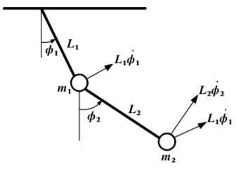
The double-pendula system comprises one plane pendulum attached to the end of another plane pendulum both oscillating in the same plane. The kinetic and potential energies for this system are given in example \(6.12.1\) to be

\[\begin{aligned}
T &=\frac{1}{2}\left(m_{1}+m_{2}\right) L_{1}^{2} \dot{\phi}_{1}^{2}+m_{2} L_{1} L_{2} \dot{\phi}_{1} \dot{\phi}_{2} \cos \left(\phi_{1}-\phi_{2}\right)+\frac{1}{2} m_{2} L_{2}^{2} \dot{\phi}_{2}^{2} \\
U &=\left(m_{1}+m_{2}\right) g L_{1}\left(1-\cos \phi_{1}\right)+m_{2} g L_{2}\left(1-\cos \phi_{2}\right)
\end{aligned} \]

a) Small-amplitude linear regime

Use of the small-angle approximation makes this system linear and solvable analytically. That is, \(T\) and \(U\) become

\[\begin{aligned}
U &=\frac{1}{2}\left(m_{1}+m_{2}\right) g L_{1} \phi_{1}^{2}+\frac{1}{2} m_{2} g L_{2} \phi_{2}^{2} \\
T &=\frac{1}{2}\left(m_{1}+m_{2}\right) L_{1}^{2} \dot{\phi}_{1}^{2}+m_{2} L_{1} L_{2} \dot{\phi}_{1} \dot{\phi}_{2}+\frac{1}{2} m_{2} L_{2}^{2} \dot{\phi}_{2}^{2}
\end{aligned} \]

Thus the kinetic energy and potential energy tensors are

\[\mathbf{T}= \begin{Bmatrix} \left(m_{1}+m_{2}\right) L_{1}^{2} & m_{2} L_{1} L_{2} \\ m_{2} L_{1} L_{2} & m_{2} L_{2}^{2} \end{Bmatrix} \quad \mathbf{V}= \begin{Bmatrix} \left( m_{1}+m_{2}\right) g L_{1} & 0 \\
0 & m_{2} g L_{2} \end{Bmatrix} \nonumber\]

Note that \(\mathbf{T}\) is nondiagonal, whereas \(\mathbf{V}\) is diagonal which is opposite to the case of the two parallel-coupled plane pendula.

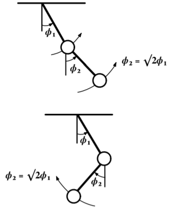
Figure \(\PageIndex{4}\): Normal modes for two series-coupled plane pendula.

The solution of this case is simpler if it is assumed that \(L_1 = L_2 = L\) and \(m_1 = m_2 = m\). Then

\[\mathbf{T} = mL^2 \begin{Bmatrix} 2 & 1 \\ 1 & 1 \end{Bmatrix} \quad \mathbf{V} = \begin{Bmatrix} 2\omega^2_0 & 0 \\ 0 & \omega^2_0 \end{Bmatrix} \nonumber\]

where \(\omega_0 = \sqrt{\frac{g}{L}}\) which is the frequency of a single pendulum.

The next stage is to evaluate the secular determinant

\[mL^2 \begin{vmatrix} 2(\omega^2_0 − \omega^2) & −\omega^2 \\ −\omega^2 & (\omega^2_0 − \omega^2) \end{vmatrix} = 0 \nonumber\]

The eigenvalues are

\[\omega^2_1 = (2 − \sqrt{2})\omega^2_0 \quad \omega^2_2 = (2 + \sqrt{ 2})\omega^2_0 \nonumber\]

As shown in the adjacent figure, the normal modes for this system are

\[\eta_1 = \frac{1}{2a_{11}} (\phi_1 + \frac{\phi_2}{\sqrt{2}} ) \quad \eta_2 = \frac{1}{2a_{22}} (\phi_1 - \frac{\phi_2}{\sqrt{2}} ) \nonumber\]

The second mass has a \(\sqrt{2}\) larger amplitude that is in phase for solution 1 and out of phase for solution 2.

b) Large amplitude chaotic regime

Stachowiak and Okada [Sta05] used computer simulations to numerically analyze the behavior of this system with increase in the oscillation amplitudes. Poincaré sections, bifurcation diagrams, and Lyapunov exponents all confirm that this system evolves from regular normal-mode oscillatory behavior in the linear regime at low energy, to chaotic behavior at high excitation energies where non-linearity dominates. This behavior is analogous to that of the driven, linearly-damped, harmonic pendulum described in chapter \(3.5\)