2.1: Introduction

The electrostatic limit is the ideal case in which nothing changes with time. All source distributions are stationary, ie \(\frac{\partial}{\partial t}\) is zero. Therefore Maxwell’s equations reduce to

\[ \begin{align} &\operatorname{curl}(\overrightarrow{\mathrm{E}})=0 \\& \operatorname{div}(\overrightarrow{\mathrm{B}})=0 \\& \operatorname{curl}(\overrightarrow{\mathrm{B}})=\mu_{0}\left(\overrightarrow{\mathrm{J}}_{f}+\operatorname{curl}(\overrightarrow{\mathrm{M}})\right) \\& \operatorname{div}(\overrightarrow{\mathrm{E}})=\frac{1}{\epsilon_{0}}\left(\rho_{f}-\operatorname{div}(\overrightarrow{\mathrm{P}})\right) \end{align} \]

Notice that the magnetic field has become totally uncoupled from the electric field. As far as the static electric field is concerned the magnetic properties of matter are irrelevant. The calculation of the static magnetic field from its sources will be the subject of Chapter(4).

Notice that −div(\(\vec P\)) is a source of the electrostatic field that is on an equal footing with the free charge density, ρ_f . The electrostatic electric field can be calculated for a given source distribution using the principle of superposition. For example, suppose that

Figure \(\PageIndex{1}\): Given a distribution of sources the electric field at the position of the observer, (X,Y,Z), can be calculated as the sum of the electric fields generated by dividing the source distribution into small volume elements dV=dxdydz and treating the charges or dipole moments in each volume element as a point charge or as a point dipole moment.

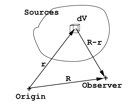
one is given a charge density distribution ρ(x,y,z), and let the observer be located at (X,Y,Z). The total charge contained within a volume element dV located at (x,y,z) is given by dQ = ρ(x,y,z)dxdydz. If dV is taken to be sufficiently small the charge dQ can be treated like a point charge. It will generate an electric field contribution at the position of the observer that is given by Coulomb’s law:

\[d\overrightarrow{\mathrm{E}}=\frac{1}{4 \pi \epsilon_{0}} d Q \frac{(\overrightarrow{\mathrm{R}}-\overrightarrow{\mathrm{r}})}{|\overrightarrow{\mathrm{R}}-\overrightarrow{\mathrm{r}}|^{3}}, \nonumber\]

where \(\vec R\) is the vector that specifies the position of the observer and \(\vec r\) is the vector that specifies the location of the volume element, dV (see Figure (2.1.1). The total electric field at the position of the observer can be calculated as the vector sum of the electric field contributions from all volume elements:

\[\overrightarrow{\mathrm{E}}(X, Y, Z)=\frac{1}{4 \pi \epsilon_{0}} \int \int \int_{A l l S p a c e} d x d y d z \rho(x, y, z) \frac{(\overrightarrow{\mathrm{R}}-\overrightarrow{\mathrm{r}})}{|\overrightarrow{\mathrm{R}}-\overrightarrow{\mathrm{r}}|^{3}}.\]

It is very seldom that the above integral can be carried out analytically. In all but a few special cases the integral must be calculated using a computer and small but finite volume elements. Equation (2.1.5) is valid even when the point of observation is located within the charge distribution so that the distance |\(\vec R\) −\(\vec r\)| goes to zero for a volume element located at the position of the observer. Why Equation (2.1.5) still works is not obvious but can be understood using the following argument. Surround the point of observation by a small sphere whose radius, R₀, is finite but is so small that the spatial variation of the charge density within the sphere can be neglected. The electric field at the observer due to charges outside the sphere of radius R₀ can be carried out without problems created by a vanishing denominator in Equation (2.1.5).

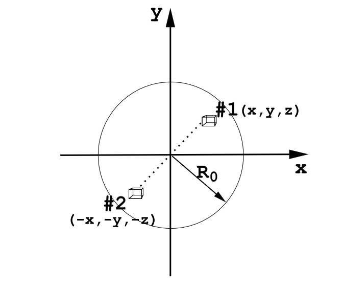
To the electric field generated by charges outside the sphere one must add the electric field generated at the center of the sphere by the charges inside the radius R₀. However, the electric field at the center of a uniformly charged sphere vanishes by symmetry, see Figure (2.1.2). For every element of charge at (x,y,z) there is a second equal element of charge at (-x,-y,-z) whose field is equal in magnitude but opposite in direction to the field of the first charge element. Thus the fields generated by these symmetry related charge pairs cancel.

2.1.1 Dipole Moment Density as a Source for the Electric Field.

A point electric dipole generates an electric field according to Equation (1.2.10). This point dipole formula can be used to calculate the electric field at some point in space, (X,Y,Z), generated by a distribution of dipole density \(\vec P\)(x,y,z). The idea is to divide up the source distribution into small volume elements, dV, and then to use the principle of superposition to obtain the electric field as the vector sum of the fields produced by the dipole moments \(\vec P\)(x,y,z)dV treated as point dipoles. The electric field at the position \(\vec R\)(X,Y,Z), the position of the observer- see Figure (2.1.1), can be written

Figure \(\PageIndex{2}\): A sphere of radius R₀ filled with a uniform charge density ρ₀. The electric field at the center of the sphere is zero because the field generated by element number 1 at (x,y,z) is cancelled by the field equal in magnitude but opposite in direction generated by the equal volume element number 2 at (-x,-y,-z). The net field generated by all such symmetry related pairs is zero.

\[\overrightarrow{\mathrm{E}}(X, Y, Z)=\frac{1}{4 \pi \epsilon_{0}} \int \int \int_{S_{p a c c}} d x d y d z\left(\frac{3[\overrightarrow{\mathrm{P}}(x, y, z) \cdot(\overrightarrow{\mathrm{R}}-\overrightarrow{\mathrm{r}})](\overrightarrow{\mathrm{R}}-\overrightarrow{\mathrm{r}})}{|\overrightarrow{\mathrm{R}}-\overrightarrow{\mathrm{r}}|^{5}}-\frac{\vec{P}(x, y, z)}{|\overrightarrow{\mathrm{R}}-\overrightarrow{\mathrm{r}}|^{3}}\right). \]

This complex formula can be seldom evaluated exactly. Usually it must be evaluated approximately by means of a computer. Eqn.(2.1.6) is valid for points of observation both inside and outside the electric dipole density distribution. If the observation point lies inside the dipole density distribution one must surround it by a small sphere of radius R0 and carry out the summations implied by Equation (2.1.6) for the space outside the sphere. This is required in order to avoid the divergence obtained when \(\vec R\) = \(\vec r\). The radius R₀ must be chosen so small that variations of the dipole density, \(\vec P\), within the sphere can be neglected. After having calculated the contribution to the electric field generated by the dipole density distribution from points outside the sphere, one must add an electric field contribution from the dipoles inside the sphere. It is not clear at this point how to calculate this contribution, but later it will be shown that the electric field at the center of a uniformly polarized sphere, polarization density \(\vec P\)₀, is given by

\[\overrightarrow{\mathrm{E}}_{0}=-\frac{\overrightarrow{\mathrm{P}}_{0}}{3 \epsilon_{0}}. \nonumber\]

This field \(\vec E\)₀ must be added to the electric field generated by the dipole sources outside the sphere of radius R₀ in order to obtain the total electric field strength at the position of the observer.

The procedure outlined above is very complicated due to the complex form of the electric field generated by a point dipole. A second, simpler approach, is suggested by the Maxwell Equation (2.1.4). Namely, one can use Equation (2.1.5) with the charge density given by

\[\rho(x, y, z)=-\operatorname{div} \overrightarrow{\mathrm{P}}(x, y, z).\]

It is clear from Equation (2.1.7) that a spatially uniform dipole moment density distribution does not generate an electric field. However, one must be careful: any dipole distribution confined to a finite region of space must vary rapidly at its surfaces. This rapid variation of the dipole density produces an effective charge density distribution that may become very large and is localized near those surfaces. These surface charge density distributions must be taken into account when calculating the electric field.