2.3: General Theorems

Last updated
Save as PDF

Page ID: 22792

\( \newcommand{\vecs}[1]{\overset { \scriptstyle \rightharpoonup} {\mathbf{#1}} } \) \( \newcommand{\vecd}[1]{\overset{-\!-\!\rightharpoonup}{\vphantom{a}\smash {#1}}} \)\(\newcommand{\id}{\mathrm{id}}\) \( \newcommand{\Span}{\mathrm{span}}\) \( \newcommand{\kernel}{\mathrm{null}\,}\) \( \newcommand{\range}{\mathrm{range}\,}\) \( \newcommand{\RealPart}{\mathrm{Re}}\) \( \newcommand{\ImaginaryPart}{\mathrm{Im}}\) \( \newcommand{\Argument}{\mathrm{Arg}}\) \( \newcommand{\norm}[1]{\| #1 \|}\) \( \newcommand{\inner}[2]{\langle #1, #2 \rangle}\) \( \newcommand{\Span}{\mathrm{span}}\) \(\newcommand{\id}{\mathrm{id}}\) \( \newcommand{\Span}{\mathrm{span}}\) \( \newcommand{\kernel}{\mathrm{null}\,}\) \( \newcommand{\range}{\mathrm{range}\,}\) \( \newcommand{\RealPart}{\mathrm{Re}}\) \( \newcommand{\ImaginaryPart}{\mathrm{Im}}\) \( \newcommand{\Argument}{\mathrm{Arg}}\) \( \newcommand{\norm}[1]{\| #1 \|}\) \( \newcommand{\inner}[2]{\langle #1, #2 \rangle}\) \( \newcommand{\Span}{\mathrm{span}}\)\(\newcommand{\AA}{\unicode[.8,0]{x212B}}\)

A number of rules, or theorems, can be deduced from Maxwell’s equations (2.1.1) and (2.1.4).

2.3.1 Application of Gauss’ Theorem

From Maxwell’s equations one has

\[\operatorname{div}(\overrightarrow{\mathrm{E}})=\frac{\rho_{t}}{\epsilon_{0}} \nonumber\]

where ρ_t = ρ_f + ρ_b, and ρ_b = −div(\(\vec P\)). Integrate Equation (2.1.4) over any closed volume V:

\[ \int \int \int_{V} d V d i v(\overrightarrow{\mathrm{E}})=\frac{1}{\epsilon_{0}} \int \int \int_{V} d V \rho_{t}=\frac{Q_{t}}{\epsilon_{0}}. \nonumber \]

But from Gauss’ Theorem, section(1.3.3)

\[\int \int \int_{V} d V d i v(\vec{E})=\int \int \int_{S} d S(\vec{E} \cdot \hat{\mathbf{n}}), \nonumber\]

where S is the surface bounding the volume V, and \(\hat{\mathbf{n}}\) is a unit vector normal to the element of surface area, dS, and directed from inside the volume to the outside. Thus the total charge \(Q_{t}=\int \int \int_{V} d V \rho_{t}\) contained within the volume V can be calculated from a knowledge of the electric field everywhere on the surface S bounding the volume V:

\[Q_{t}=\epsilon_{0} \int \int_{S} d S(\overrightarrow{\mathrm{E}} \cdot \hat{\mathbf{n}}). \label{2.16}\]

It is often useful to rewrite Equation (2.1.4) in terms of the displacement vector \(\overrightarrow{\mathrm{D}}=\epsilon_{0} \overrightarrow{\mathrm{E}}+\overrightarrow{\mathrm{P}}\). Notice that \(\vec D\) and \(\vec P\) have the same units, Coulombs/m² , and these units are different from the electric field units of Volts/m. Using the above definition of \(\vec D\) the fourth Maxwell equation becomes

\[\operatorname{div}(\overrightarrow{\mathrm{D}})=\rho_{f}, \label{2.17}\]

where ρ_f is the density of free charges. Integrate Equation (\ref{2.17}) over a volume V and apply Gauss’ Theorem to obtain

\[\int \int \int_{V} d V d i v(\overrightarrow{\mathrm{D}})=\int \int_{S} d S(\overrightarrow{\mathrm{D}} \cdot \hat{\mathbf{n}})=\int \int \int_{V} d V \rho_{f}. \nonumber \]

It follows from this that the total free charge within a volume V can be calculated from a knowledge of the displacement vector, \(\vec D\), over the surface S bounding the volume V:

\[Q_{f}=\iint_{S} d S(\overrightarrow{\mathrm{D}} \cdot \hat{\mathbf{n}}). \label{2.18}\]

2.3.2 Boundary Condition on \(\vec D\).

Gauss’ theorem in the form of Equation (\ref{2.18}) can be used to show that the normal component of the displacement vector, \(\vec D\), must be continuous at the boundary between two different materials if that boundary contains no free surface charges. Refer to Figure (2.3.4). Let SS be the surface that separates region (1) from region (2). Apply Equation (\ref{2.18}) to a pill-box that straddles the bounding surface SS. The surface area of the pill-box is ∆S and it is dL thick: the thickness dL will be taken to be small compared with the lateral dimensions of the pill-box, ∼ \(\sqrt{\Delta S}\). The contribution to the surface integral in (\ref{2.18}) from the sides of the pill-box will be negligible because (1) its area will be very small since dL is relatively small, and (2) the components of \(\overrightarrow{\mathrm{D}}_{1}, \overrightarrow{\mathrm{D}}_{2}\) parallel with the surface SS, the tangential components, will be very nearly constant over the dimensions of the pill-box and so as the outward

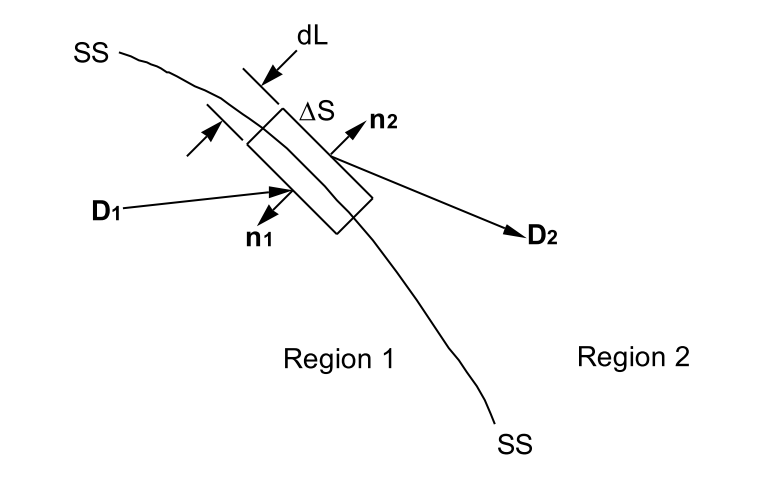
Figure 2.4.PNG — Figure \(\PageIndex{4}\): Application of Gauss’ Theorem to a pill-box straddling a surface of discontinuity between two materials.

normal changes direction by 360 degrees around the pill-box perimeter the positive and negative contributions to the surface integral will cancel. Thus in the limit as dL → 0 and ∆A → 0 the surface integral taken over the pill-box surface will be given by

\[\int \int_{\text {Pill-box}} d S(\overrightarrow{\mathrm{D}} \cdot \hat{\mathbf{n}})=\left(\overrightarrow{\mathrm{D}}_{2} \cdot \hat{\mathbf{n}}_{2}\right) \Delta A+\left(\overrightarrow{\mathrm{D}}_{1} \cdot \hat{\mathbf{n}}_{1}\right) \Delta A. \nonumber \]

But \(\overrightarrow{\mathrm{D}}_{2} \cdot \hat{\mathbf{n}}_{2}=+D_{2 n}\) and \(\overrightarrow{\mathrm{D}}_{1} \cdot \hat{\mathbf{n}}_{1}=-D_{n 1}\) where D_2n, D_1n are the components of \(\overrightarrow{\mathrm{D}}_{2}\), \(\overrightarrow{\mathrm{D}}_{1}\) normal to the bounding surface SS. It follows from Gauss’ theorem, Equation (\ref{2.18}), that if there are no free charge densities in the two materials then the total charge contained in the pill-box is zero and therefore D_2n−D_1n = 0, so that the normal component of D must be continuous across the bounding surface SS. This result remains valid even if the volume density of free charges is not zero because the total charge contained in the pill-box of Figure (2.3.4) goes to zero as the pill-box volume goes to zero with the pill-box thickness, dL. The normal component of \(\vec D\) can only be discontinuous if the surface SS carries a surface charge density. If the bounding surface SS carries a surface charge density of σ_f Coulombs/m² the total charge contained within the pill-box of Figure (2.3.4) is σ_f∆A Coulombs, and Equation (\ref{2.18}) gives

\[D_{2 n} \Delta A-D_{1 n} \Delta A=\sigma_{f} \Delta A\nonumber \]

since the charge contained within the pill-box, σ_f∆A, is independent of dL, and does not vanish as dL → 0. It follows that any discontinuity in the normal component of the displacement vector D is an indication and a measure of the presence of a surface charge density:

\[\sigma_{f}=D_{2 n}-D_{1 n}. \label{2.19} \]

2.3.3 Discontinuity in the Normal Component of the Polarization Vector.

Gauss’ theorem can be used to show that a discontinuity in the normal component of the electrical polarization vector, \(\vec P\), produces a surface density of bound charges, σ_b. Consider a surface that separates regions having different material properties such as that shown in Figure (2.3.4), and in particular two regions having different polarization densities \(\vec P\)₁ and \(\vec P\)₂. Let there be no free charge distributions, and let there be no free charges on the surface of discontinuity, SS. For this situation Equation (2.1.4) becomes

\[\operatorname{div}(\overrightarrow{\mathrm{E}})=-\frac{1}{\epsilon_{0}} \operatorname{div}(\overrightarrow{\mathrm{P}})=\frac{\rho_{b}}{\epsilon_{0}}. \nonumber \]

Apply Gauss’ theorem to this equation for a pill-box straddling the boundary SS such as that illustrated in Figure (2.3.4). In the limit as dL → 0 and ∆A → 0 the surface integral over the pill-box of the electric field gives

\[\int \int_{P i l l-b o x} d S(\overrightarrow{\mathrm{E}} \cdot \hat{\mathbf{n}})=\left(\overrightarrow{\mathrm{E}}_{2} \cdot \hat{\mathbf{n}}_{2}\right) \Delta A+\left(\overrightarrow{\mathrm{E}}_{1} \cdot \hat{\mathbf{n}}_{1}\right) \Delta A.\nonumber \]

But \(\overrightarrow{\mathrm{E}}_{2} \cdot \hat{\mathbf{n}}_{2}=E_{2 n}\), and \(\overrightarrow{\mathrm{E}}_{1} \cdot \hat{\mathbf{n}}_{1}=-E_{1 n}\) where E_2n and E_1n are the components of the electric field normal to the bounding surface SS. Thus

\[\int \int \int_{\text {Pill-box }} d V d i v(\overrightarrow{\mathrm{E}})=\frac{1}{\epsilon_{0}} \int \int \int_{\text {Pill-box }} d V \rho_{b}=\frac{Q_{b}}{\epsilon_{0}} \nonumber \]

and Gauss’ Theorem gives

\[\int \int_{P i l l-b o x} d S(\overrightarrow{\mathrm{E}} \cdot \hat{\mathbf{n}})=\left(E_{2 n}-E_{1 n}\right) \Delta A=\frac{Q_{b}}{\epsilon_{0}}. \nonumber \]

Q_b is the total bound charge contained in the pill-box. As the thickness of the pill-box shrinks to zero the only bound charges left in the pill-box will be due to surface bound charges, σ_b, and therefore Q_b = σ_b∆A. It follows that

\[\sigma_{b}=\epsilon_{0}\left(E_{2 n}-E_{1 n}\right). \label{2.20} \]

This equation (\ref{2.20}) is the analog of Equation (\ref{2.19}) and the derivations of these two equations are similar. In the present case it has been assumed that there are no free surface charges on the interface surface SS so that from Equation (\ref{2.19}) one has (D_2n − D_1n) = 0 and therefore from the definition of \(\vec D\)

\[D_{2 n}-D_{1 n}=\left(\epsilon_{0} E_{2 n}+P_{2 n}\right)-\left(\epsilon_{0} E_{1 n}+P_{1 n}\right)=0. \nonumber \]

Using Equation (\ref{2.20}) gives

\[\sigma_{b}=-\left(P_{2 n}-P_{1 n}\right). \label{2.21} \]

Any discontinuity in the normal component of the Polarization vector generates a surface density of bound charges. These bound charges generate electric fields and must be explicitly taken into account when the electric field is calculated from its sources using Equation (2.1.5), (the direct application of Coulomb’s law), or when Equation (2.2.6) is used to calculate the potential function for a distribution of free and bound charges.