4.2: The Law of Biot-Savart

It often happens that the current density is confined to a relatively small cross-section. Consider, for example, the case of a thin wire carrying a current, see Figure (4.1.2). For this case the current density is I/S inside the wire, where S is the cross-sectional area of the wire, and the current density is zero outside the wire. If the thickness of the wire is very small compared with the distance to the point of observation, one can neglect the very small variations of \(|\overrightarrow{\mathrm{R}}-\overrightarrow{\mathrm{r}}|=\sqrt{(\mathrm{X}-\mathrm{x})^{2}+(\mathrm{Y}-\mathrm{y})^{2}+(\mathrm{Z}-\mathrm{z})^{2}}\) for the various elements across the wire section, so that when integrated over the wire cross-section Equations (4.1.14) and (4.1.15) become line integrals:

\[\vec{A}_{P}=\frac{\mu_{0} I}{4 \pi} \int_{W i r e} \frac{d \vec{L}}{|\vec{r}|}, \label{4.16}\]

Figure \(\PageIndex{3}\): Derivation of the law of Biot-Savart from the fields generated by a slowly moving point charge.

and

\[\overrightarrow{\mathrm{B}}_{P}=\frac{\mu_{0} \mathrm{I}}{4 \pi} \int_{\text {Wire }} \frac{(\overrightarrow{\mathrm{d}} \overrightarrow{\mathrm{L}} \times \overrightarrow{\mathrm{r}})}{|\overrightarrow{\mathrm{r}}|^{3}}. \label{4.17}\]

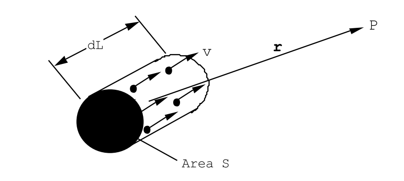
Equation (\ref{4.17}) is called the law of Biot-Savart. Notice that the magnetic fieldstrength falls off like 1/r² with distance from a small element of current. The law of Biot-Savart can also be deduced directly from the expression for the magnetic field generated by a slowly moving point charge, Chapter(1), Equation (1.1.7). Consider a small element of a wire containing N charges q per unit volume that are moving along the wire with a velocity v, see Figure (4.2.3). The charge density contributed by the mobile charge carriers are supposed to be exactly compensated by an equal number density of fixed charges of opposite sign. The current flowing through the wire is numerically equal to the charge contained in a cylinder of area S and equal in length to the velocity, v: all of the mobile charges in such a cylinder will pass through a given cross-section in 1 second,

\[\mathrm{I}=\mathrm{NSq}_{\mathrm{V}} \quad \text { Ampères }. \label{4.18}\]

The electric field due to the mobile charge carriers contained in a piece of wire dL long is just given by

\[\overrightarrow{\mathrm{dE}}_{P}=\frac{1}{4 \pi \epsilon_{0}} \mathrm{NSqdL} \frac{\overrightarrow{\mathrm{r}}}{|\overrightarrow{\mathrm{r}}|^{3}}. \nonumber \]

These charges produce a magnetic field because of their motion

\[\mathrm{d} \overrightarrow{\mathrm{B}}_{P}=\frac{1}{c^{2}}\left[\overrightarrow{\mathrm{v}} \times \overrightarrow{\mathrm{dE}}_{P}\right]=\frac{1}{4 \pi \epsilon_{0} c^{2}} \mathrm{NSqdL} \frac{[\overrightarrow{\mathrm{v}} \times \overrightarrow{\mathrm{r}}]}{|\overrightarrow{\mathrm{r}}|^{3}}. \nonumber \]

The compensating stationary charges produce no magnetic field because their velocity relative to the observer is zero. They do, however, produce an electric field that cancels the electric field due to the mobile charges. Now use the fact that \(\vec v\) and d\(\vec L\) are parallel, along with Equation (\ref{4.18}), to obtain

\[\overrightarrow{\mathrm{dB}}_{P}=\frac{I}{4 \pi \epsilon_{0} c^{2}} \frac{[\mathrm{d} \overrightarrow{\mathrm{L}} \times \overrightarrow{\mathrm{r}}]}{|\overrightarrow{\mathrm{r}}|^{3}}. \nonumber \]

This leads directly to the integral expression Equation (\ref{4.17}) for the law of Biot and Savart since \(c^{2}=1 / \epsilon_{0} \mu_{0}\).