4.3: Standard Problems

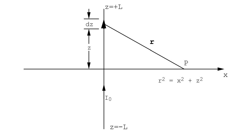
4.3.1 A Long Straight Wire.

Each element of the wire, d\(\vec L\), is directed along z, and therefore A has only a z-component, see Figure (4.3.4) and Equation (4.1.16):

\[\mathrm{d} \mathrm{A}_{\mathrm{z}}=\frac{\mu_{0}}{4 \pi} \frac{\mathrm{I}_{0} \mathrm{d} \mathrm{z}}{\sqrt{\mathrm{z}^{2}+\mathrm{x}^{2}}}. \label{4.19}\]

Unfortunately, the integral of Equation (\ref{4.19}) diverges if it is evaluated over the interval −∞ ≤ z ≤ ∞ . This indicates that an infinitely long wire is unphysical; eventually the two ends of the wire must be connected in order to complete the steady state current loop. In order to proceed, one can calculate the contribution to the vector potential from the large but finite wire segment −L ≤ z ≤ +L. The result is

\[\mathrm{A}_{\mathrm{z}}(\mathrm{x})=\frac{\mu_{0} \mathrm{I}_{0}}{4 \pi} \ln \left(\frac{\sqrt{\mathrm{L}^{2}+\mathrm{x}^{2}}+\mathrm{L}}{\sqrt{\mathrm{L}^{2}+\mathrm{x}^{2}}-\mathrm{L}}\right). \nonumber \]

Clearly A_z must have the same value everywhere on a circle of radius x centered on the origin and lying in the x-y plane. The expression for the

Figure \(\PageIndex{4}\): A straight wire 2L meters long, and carrying a current of I₀ Amp`eres, used to calculate the vector potential and the magnetic field generated at a point P in the central plane.

vector potential may therefore be written in cylindrical polar co-ordinates as

\[\mathrm{A}_{\mathrm{z}}(\mathrm{r})=\frac{\mu_{0} \mathrm{I}_{0}}{4 \pi} \ln \left(\frac{\sqrt{\mathrm{L}^{2}+\mathrm{r}^{2}}+\mathrm{L}}{\sqrt{\mathrm{L}^{2}+\mathrm{r}^{2}}-\mathrm{L}}\right). \nonumber \]

Although this expression is strictly valid only for points in the x-y plane, it is clear from symmetry arguments that for large L and small z the vector potential must be essentially independent of z. The corresponding magnetic field is given by \(\vec B\) = curl(\(\vec A\)), and since \(\vec A\) has only a z-component, and since this z-component is independent of the angle θ, the magnetic field has only a θ-component:

\[\mathrm{B}_{\theta}=-\left(\frac{\partial \mathrm{A}_{z}}{\partial \mathrm{r}}\right)=\frac{\mu_{0} \mathrm{I}_{0}}{2 \pi} \frac{\mathrm{L}}{\mathrm{r} \sqrt{\mathrm{L}^{2}+\mathrm{r}^{2}}}. \nonumber \]

If L ≫ r this expression reduces to

\[\mathrm{B}_{\theta}=\frac{\mu_{0} \mathrm{I}_{0}}{2 \pi} \frac{1}{\mathrm{r}}. \label{4.20}\]

4.3.2 A Long Straight Wire Revisited.

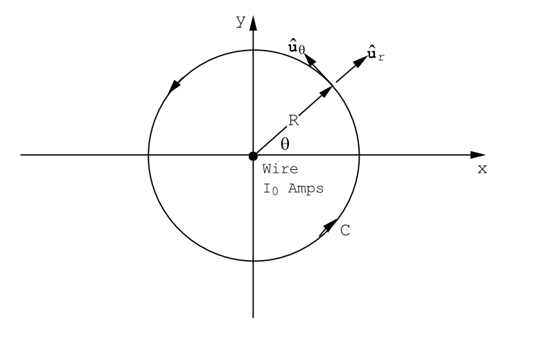
The result Equation (\ref{4.20}) for the magnetic field generated by a long straight wire is so simple that it suggests that there must be an easy method for obtaining it: a method based upon the symmetry of the problem. Magnetic problems in which the current distribution is very symmetric may often be solved by means of an application of Stokes’ theorem (Chpt.(1), Section(1.3.4)). Stokes’ theorem states that the surface integral of the curl of any vector field over a surface bounded by a closed curve C can be replaced by the line integral of that vector over the curve C. Apply this theorem to the Maxwell equation

\[\operatorname{curl}(\overrightarrow{\mathrm{B}})=\mu_{0}\left(\overrightarrow{\mathrm{J}}_{\mathrm{f}}+\operatorname{curl}(\overrightarrow{\mathrm{M}})\right)=\mu_{0} \overrightarrow{\mathrm{J}}_{\mathrm{T}}. \nonumber \]

For the present problem there is no magnetization density; \(\overrightarrow{\mathrm{M}}=0\) everywhere and therefore \(\operatorname{curl}(\overrightarrow{\mathrm{M}})=0\) everywhere and \(\overrightarrow{\mathrm{J}}_{\mathrm{T}}=\overrightarrow{\mathrm{J}_{\mathrm{f}}}\). The current flow is confined to the cross-section of the wire so that if one applies Stokes’ theorem to the surface bounded by the circle of radius R shown in Figure (4.3.5) one obtains

\[\iint_{S u r f a c e} \operatorname{dScurl}(\overrightarrow{\mathrm{B}}) \cdot \hat{\mathbf{n}}=\mu_{0} \iint_{\text {Surface}} \mathrm{dS} \overrightarrow{\mathrm{J}}_{\mathrm{f}} \cdot \hat{\mathbf{n}}=\mu_{0} \mathrm{I}_{0}, \nonumber \]

Figure \(\PageIndex{5}\): Geometry used to calculate the magnetic field generated by a long straight wire carrying a current of I₀ Amp`eres.

where dS is the element of area, and \(\hat{\mathbf{n}}\) is a unit vector normal to the element of surface area. But from Stokes’ Theorem

\[\iint_{S u r f a c e} \operatorname{dS} \operatorname{curl}(\overrightarrow{\mathrm{B}}) \cdot \hat{\mathbf{n}}=\oint_{C} \overrightarrow{\mathrm{B}} \cdot \mathrm{d} \overrightarrow{\mathrm{L}}, \nonumber \]

\[\oint_{C} \overrightarrow{\mathrm{B}} \cdot \overrightarrow{\mathrm{d}}=\mu_{0} \mathrm{I}_{0}. \nonumber \]

The law of Biot-Savart, Equation (4.1.17), can be used to convince oneself that \(\vec B\) has only a component in the direction tangent to the circle C of Figure (4.3.5). By symmetry this component must be independent of position along the circumference of the circle, and the line integral in is very easy to carry out.

\[\oint_{C} \overrightarrow{\mathrm{B}} \cdot \mathrm{d} \overrightarrow{\mathrm{L}}=2 \pi \mathrm{RB}_{\theta}=\mu_{0} \mathrm{I}_{0}, \nonumber \]

or

\[\mathrm{B}_{\theta}=\frac{\mu_{0} \mathrm{I}_{0}}{2 \pi \mathrm{R}}, \label{4.21}\]

Figure \(\PageIndex{6}\): The magnetic field generated along the axis of a circular current loop.

in agreement with Equation (\ref{4.20}) deduced from the vector potential. Unfortunately, most problems do not exhibit sufficient symmetry to be so simply solved.

4.3.3 A Circular Loop.

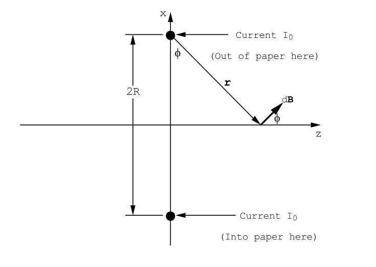
Refer to Figure (4.3.6). In this case the field is most simply calculated by direct application of the law of Biot-Savart, Equation (4.1.17). The element of magnetic field, d\(\vec B\), generated by any small element of length, d\(\vec L\), along the wire is perpendicular both to d\(\vec L\) and to \(\vec r\) as shown in Figure (4.3.6). The transverse component of d\(\vec B\) is cancelled by symmetry by the contribution from the element of length that is diametrically opposite to d\(\vec L\). Thus along the axis of the loop there is only a z-component of magnetic field:

\[\mathrm{dB}_{\mathrm{z}}=\frac{\mu_{0} \mathrm{I}_{0}}{4 \pi}\left(\frac{\mathrm{dL}}{\mathrm{r}^{2}}\right) \cos \phi=\frac{\mu_{0} \mathrm{I}_{0}}{4 \pi} \frac{\mathrm{RdL}}{\mathrm{r}^{3}}. \nonumber \]

Figure \(\PageIndex{7}\): The magnetic field along the axis of a solenoid L meters long, R meters in radius, and having N turns per meter.

This expression can be readily integrated because the distance r does not depend upon position around the circumference of the wire. Thus

\[\mathrm{B}_{\mathrm{z}}=\frac{\mu_{0} \mathrm{I}_{0}}{4 \pi}\left(\frac{\mathrm{R}}{\mathrm{r}^{3}}\right) \oint_{C} \mathrm{d} \overrightarrow{\mathrm{L}}=\frac{\mu_{0} \mathrm{I}_{0}}{2} \frac{\mathrm{R}^{2}}{\left[\mathrm{z}^{2}+\mathrm{R}^{2}\right]^{3 / 2}}. \label{4.22}\]

This expression, together with the principle of superposition, can be used to calculate the magnetic field along the axis of a solenoid.

4.3.4 The Magnetic Field along the Axis of a Solenoid.

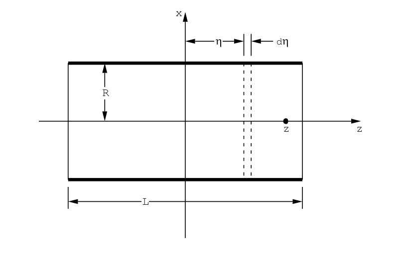
Consider a coil L meters long that is uniformly wound with N turns/meter. The magnetic field at a point on the axis of the coil can be calculated as the sum of the fields generated by each turn separately using the principle of superposition. The field generated by a single turn located at \(\eta\) is given by

\[\mathrm{B}_{\mathrm{z}}=\left(\frac{\mu_{0} \mathrm{I}_{0} \mathrm{R}^{2}}{2}\right) \frac{1}{\left((\mathrm{z}-\eta)^{2}+\mathrm{R}^{2}\right)^{3 / 2}}, \nonumber \]

where I₀ is the current; this follows from Equation (\ref{4.22}). The field generated at z by the \(\mathrm{N} d \eta\) turns contained in the element of length \(d \eta\) is given by

\[\mathrm{dB}_{\mathrm{z}}=\left(\frac{\mu_{0} \mathrm{I}_{0} \mathrm{R}^{2}}{2}\right) N \frac{d \eta}{\left((\mathrm{z}-\eta)^{2}+\mathrm{R}^{2}\right)^{3 / 2}}. \nonumber \]

Upon integration over \(\eta\) the total field becomes

\[\mathrm{B}_{\mathrm{z}}=\left(\frac{\mu_{0} \mathrm{I}_{0} \mathrm{R}^{2} \mathrm{N}}{2}\right) \int_{-L / 2}^{L / 2} \frac{d \eta}{\left((\mathrm{z}-\eta)^{2}+\mathrm{R}^{2}\right)^{3 / 2}}. \nonumber \]

This is a standard integral:

\[\mathrm{B}_{z}=\left(\frac{\mu_{0} \mathrm{I}_{0} \mathrm{N}}{2}\right)\left[\frac{([\mathrm{L} / 2]+\mathrm{z})}{\sqrt{([\mathrm{L} / 2]+\mathrm{z})^{2}+\mathrm{R}^{2}}}+\frac{([\mathrm{L} / 2]-\mathrm{z})}{\sqrt{([\mathrm{L} / 2]-\mathrm{z})^{2}+\mathrm{R}^{2}}}\right]. \label{4.23}\]

The calculation of the field strength at an off-axis position is more difficult, and must be carried out numerically. In the limit as L becomes very large, ie. (z/L)≪ 1, the z dependence drops out to give

\[\mathrm{B}_{z} \rightarrow \mu_{0} \mathrm{NI}_{0}\left(\frac{\mathrm{L} / 2}{\sqrt{(\mathrm{L} / 2)^{2}+\mathrm{R}^{2}}}\right) \rightarrow \mu_{0} \mathrm{NI}_{0} \quad \text { if }(\mathrm{R} / \mathrm{L}) \ll 1. \label{4.24}\]

(Note that N is not the total number of turns on the solenoid but is the total number of turns divided by the length L.)

4.3.5 The Magnetic Field of an Infinite Solenoid.

The field in an infinite solenoid cannot depend upon position along z because the coil appears the same to a fixed observer even if it is shifted along its axis through any finite interval, ∆z. The current flow in the solenoid turns is transverse to the solenoid axis, therefore according to the expression (4.2.1) for the vector potential, \(\vec A\) must be purely transverse; ie. the vector potential \(\vec A\) can have only the components A_r and A_θ when written in cylindrical polar co-ordinates. These components cannot depend upon the angle θ because any rotation of the solenoid around its axis leaves the current distribution unchanged. The curl of a vector that has only the components A_r and A_θ,

Figure \(\PageIndex{8}\): Diagram to illustrate the use of Stokes’ Theorem to show that the field outside an infinite solenoid is zero.

and for which these components depend only upon the radial co-ordinate,r, has only a z-component,

\[\mathrm{B}_{\mathrm{z}}=\operatorname{curl}(\overrightarrow{\mathrm{A}})_{z}=\frac{1}{\mathrm{r}} \frac{\partial\left(\mathrm{r} \mathrm{A}_{\theta}\right)}{\partial \mathrm{r}}. \nonumber\]

We conclude, therefore, that the magnetic field can have only one component, B_z, and that component can depend only upon the distance r from the solenoid axis. Further note that everywhere inside the solenoid curl(\(\vec B\)) = 0 from Maxwell’s equations since there is no free current density and no magnetization density by hypothesis. But since \(\vec B\) has only a z-component that is independent of θ and z, its curl has only the component

\[\operatorname{curl}(\overrightarrow{\mathrm{B}})_{\theta}=-\frac{\partial \mathrm{B}_{z}}{\partial \mathrm{r}}=0 \nonumber \]

and therefore B_z is independent of the distance from the solenoid axis. A similar line of argument applies equally to the region outside the solenoid. It follows from Equation (\ref{4.24}), the expression for the field at the center of a long solenoid, that the field everywhere inside an infinite solenoid must be given by

\[\mathrm{B}_{z}=\mu_{0} \mathrm{NI}_{0} \quad \text { Teslas }. \label{4.25}\]

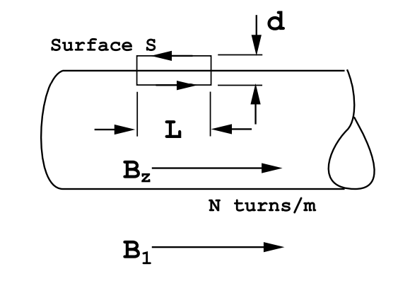
As was shown above, outside the infinite solenoid the field must be a constant, B_z = B₁ say. The value of B₁ may be calculated by means of Stokes’ theorem, Figure (4.3.8). Apply Stokes’ theorem to an area bounded by the rectangle L long and d wide that is oriented perpendicular to the current flow in the windings. From Maxwell’s equations

\[\operatorname{curl}(\overrightarrow{\mathrm{B}})=\mu_{0} \overrightarrow{\mathrm{J}}_{\mathrm{f}}, \nonumber \]

since there is no magnetization density and the fields are static. Therefore

\[\int \int_{S} \mathrm{dS} \operatorname{curl}(\overrightarrow{\mathrm{B}}) \cdot \hat{\mathbf{n}}=\mu_{0} \iint_{S} \mathrm{dS} \overrightarrow{\mathrm{J}}_{\mathrm{f}} \cdot \hat{\mathbf{n}}=\mu_{0} \mathrm{NI}_{0} \mathrm{L}. \nonumber \]

This last result follows because \(\vec J\)_f = 0 except on the cross-section of each wire. But, referring to Figure (4.3.8)

\[\int \int_{S} \mathrm{dS} \operatorname{curl}(\overrightarrow{\mathrm{B}}) \cdot \hat{\mathbf{n}}=\oint_{C} \overrightarrow{\mathrm{B}} \cdot \mathrm{d} \overrightarrow{\mathrm{L}}=\mathrm{B}_{\mathrm{z}} \mathrm{L}-\mathrm{B}_{1} \mathrm{L}. \nonumber \]

The sides of the loop d meters long contribute nothing because they are perpendicular to the magnetic field. It can therefore be concluded that

\[ \left(\mathrm{B}_{\mathrm{z}}-\mathrm{B}_{1}\right)=\mu_{0} \mathrm{NI}_{0}.\label{4.26}\]

But inside the solenoid the field is B_z = µ₀NI₀, and Equation (\ref{4.26}) then requires that the field outside the solenoid be zero. The fields generated by an infinitely long solenoid are zero everywhere outside the solenoid, and a uniform field parallel with the axis, B_z = µ₀NI₀, everywhere inside the solenoid.

4.3.6 The Field generated by a Point Magnetic Dipole.

Consider a current loop of radius a meters centered on the origin and lying in the x-y plane as shown in Figure (4.3.9). For simplicity, let the point of observation, P, lie in the y-z plane; this assumption involves no loss of generality because the vector potential and the field must be independent of angle around the z-axis. The contribution of the line element \(\overrightarrow{\mathrm{d} \mathrm{L}}=a d \phi\left[-\sin \phi \hat{\mathbf{u}}_{x}+\cos \phi \hat{\mathbf{u}}_{y}\right]\) to the vector potential at P(0,Y,Z) is

\[\mathrm{d} \overrightarrow{\mathrm{A}}_{\mathrm{P}}=\frac{\mu_{0} \mathrm{I}_{0}}{4 \pi} \frac{\mathrm{d} \overrightarrow{\mathrm{L}}}{|\overrightarrow{\mathrm{R}}-\overrightarrow{\mathrm{a}}|}=\frac{\mu_{0} \mathrm{I}_{0}}{4 \pi} \text { a d } \frac{\left(-\sin \phi \hat{\mathbf{u}}_{x}+\cos \phi \hat{\mathbf{u}}_{y}\right)}{|\overrightarrow{\mathrm{R}}-\overrightarrow{\mathrm{a}}|}. \nonumber \]

Figure \(\PageIndex{9}\): Calculation of the vector potential generated by a current loop of radius a carrying a current of I₀ Amps.

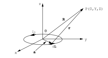
As usual \(\hat{\mathbf{u}}_{x}\) and \(\hat{\mathbf{u}}_{y}\) are unit vectors directed along x and y.

\[|\overrightarrow{\mathrm{R}}-\overrightarrow{\mathrm{a}}|=\sqrt{\mathrm{a}^{2} \cos \phi^{2}+[\mathrm{Y}-\mathrm{a} \sin \phi]^{2}+\mathrm{Z}^{2}}, \nonumber \]

or

\[ |\overrightarrow{\mathrm{R}}-\overrightarrow{\mathrm{a}}|=\mathrm{R} \sqrt{1-\frac{2 \mathrm{aY} \sin \phi}{\mathrm{R}^{2}}+\frac{\mathrm{a}^{2}}{\mathrm{R}^{2}}}, \nonumber \]

where R² = Y² + Z². Using the binomial expansion theorem along with the condition (a/R) ≪ 1 one finds, to first order in (a/R),

\[\overrightarrow{\mathrm{dA}}_{P}=\frac{\mu_{0} \mathrm{I}_{0}}{4 \pi} \frac{\mathrm{ad} \phi}{\mathrm{R}}\left(-\sin \phi \hat{\mathbf{u}}_{x}+\cos \phi \hat{\mathbf{u}}_{y}\right)\left(1+\frac{\mathrm{aY} \sin \phi}{\mathrm{R}^{2}}\right). \nonumber \]

Integrate over the angle \(\phi\) from \(\phi\) = 0 to \(\phi\) = 2\(\pi\). The integrals over sin \(\phi\), cos (\(\phi\)), and sin (\(\phi\)) cos (\(\phi\)) all vanish. However, the integral over sin (\(\phi\)²⁾ gives \(\pi\). Thus \(\vec A\)_P will have only a component parallel with the x-axis for the above choice of P lying in the Y-Z plane at (0,Y,Z):

\[\mathrm{A}_{\mathrm{x}}=-\frac{\mu_{0}}{4 \pi}\left(\pi \mathrm{a}^{2} \mathrm{I}_{0}\right) \frac{Y}{\mathrm{R}^{3}}. \nonumber \]

This result indicates, because of the symmetry around the z-axis, that in spherical polar co-ordinates the vector potential has only one component, A_\(\phi\). Let \(\mathrm{m}=\pi \mathrm{a}^{2} \mathrm{I}_{0}\); then

\[\mathrm{A}_{\phi}=\frac{\mu_{0}}{4 \pi} \frac{\mathrm{m} \sin \theta}{\mathrm{R}^{2}}. \nonumber\]

In vector notation this result can be written

\[\overrightarrow{\mathrm{A}}_{d i p}=\frac{\mu_{0}}{4 \pi} \frac{(\overrightarrow{\mathrm{m}} \times \overrightarrow{\mathrm{R}})}{\mathrm{R}^{3}} \quad \text { Tesla }-\text { meters }, \label{4.27}\]

where \(|\overrightarrow{\mathrm{m}}|=\mathrm{I}_{0} \mathrm{A}\), and \(\mathrm{A}=\pi \mathrm{a}^{2}\), the area of the current loop. It can be shown that this same result is obtained for any small current loop, whatever its shape may be, in the limit as the dimensions of the loop become very small compared with the distance to the point of observation, R.

It is simple, but tedious, to show that the magnetic field corresponding to Equation (\ref{4.27}) is given by

\[\overrightarrow{\mathrm{B}}_{\text {dip}}=\operatorname{curl}\left(\overrightarrow{\mathrm{A}}_{\text {dip}}\right)=\frac{\mu_{0}}{4 \pi}\left(\frac{3[\overrightarrow{\mathrm{m}} \cdot \overrightarrow{\mathrm{R}}] \overrightarrow{\mathrm{R}}}{\mathrm{R}^{5}}-\frac{\overrightarrow{\mathrm{m}}}{\mathrm{R}^{3}}\right). \label{4.28}\]

This result can best be obtained by calculating the curl using cartesian coordinates. Eqn.(\ref{4.28}) for the magnetic field generated by a magnetic point dipole has exactly the same form as Equation (1.2.10), the electric field produced by an electric point dipole.

4.3.7 A Long Uniformly Magnetized Rod.

Let a cylindrical rod be magnetized uniformly along its axis. Inside the rod the magnetization density, M_z = M₀, is independent of position, ie. \(\partial \mathrm{M}_{\mathrm{z}} / \partial \mathrm{r}=0\), \(\partial \mathrm{M}_{\mathrm{z}} / \partial \phi=0\) and \(\partial \mathrm{M}_{z} / \partial z=0\). Therefore, curl (\(\vec M\)) = 0 everywhere inside the rod. Similarly, curl (\(\vec M\)) = 0 everywhere outside the rod. However, curl (\(\vec M\)) does not vanish on the surface of the rod, see Figure (4.3.10). In cylindrical polar co-ordinates one finds only one non-zero component, \(\operatorname{curl}(\overrightarrow{\mathrm{M}})_{\theta}=-\partial \mathrm{M}_{2} / \partial \mathrm{r}\) the radial component of curl (\(\vec M\)) is zero because the magnetization density does not depend upon the azimuthal angle, \(\phi \). Notice that ∂M_z/∂r is zero everywhere except on the surface where M_z varies rapidly from M₀ on the inside to M_z = 0 on the outside of the rod. This rapid radial variation of M_z introduces an integrable singularity into the angular component of curl (\(\vec M\)):

\[\operatorname{curl}(\overrightarrow{\mathrm{M}})_{\theta}=-\frac{\partial \mathrm{M}_{z}}{\partial \mathrm{r}}=\mathrm{M}_{0} \delta(\mathrm{r}-\mathrm{R}). \nonumber \]

where \(\delta(\mathrm{r}-\mathrm{R})\) is the Dirac \(\delta\)-function that vanishes except at the radius r=R. The quantity curl (\(\vec M\)) is equivalent to a real current density as far as

Figure \(\PageIndex{10}\): A long cylindrical rod magnetized along the axis.

Figure \(\PageIndex{11}\): A uniformly magnetized disc.

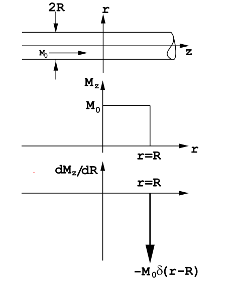
producing a magnetic field is concerned. The above surface current density produces exactly the same magnetic fields as a surface current sheet having a strength of M₀ Amps/meter; in terms of the windings on a solenoid, it is equivalent to N turns/meter carrying a current of I₀ Amps where NI₀ = M₀ Amps/meter. The field inside a uniformly magnetized rod is given by the infinite solenoid formula, Equation (\ref{4.25}),

\[\mathrm{B}_{\mathrm{z}}=\mu_{0} \mathrm{M}_{0} \quad \text { Teslas. }. \label{4.29}\]

Unfortunately this field is not accessible. The field outside an infinitely long magnetized rod is zero.

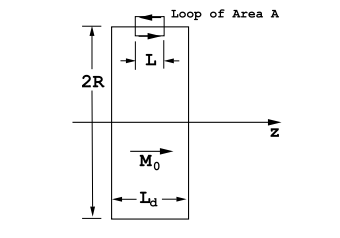
4.3.8 A Uniformly Magnetized Disc.

The discontinuity in the tangential component of the magnetization density at the surfaces of a uniformly magnetized disc produces an effective surface current density that sets up a magnetic field whose distribution is exactly equivalent to the field set up by a solenoid of the same length. The strength of the effective current sheet is M₀ Amps/meter, and is equivalent to N turns/meter carrying I₀ Amps, where NI₀ = M₀. This can be shown using Stokes’ Theorem applied to a small loop of area A that spans the surface of the disc as shown in Figure (4.3.11). The field along the axis of a disc of thickness Ld is given by Equation (\ref{4.23}) applied to this case :

\[\mathrm{B}_{z}=\frac{\mu_{0} \mathrm{M}_{0}}{2}\left(\frac{\left[\left(\mathrm{L}_{\mathrm{d}} / 2\right)+z\right]}{\sqrt{\left[\left(\mathrm{L}_{\mathrm{d}} / 2\right)+z\right]^{2}+\mathrm{R}^{2}}}+\frac{\left[\left(\mathrm{L}_{\mathrm{d}} / 2\right)-z\right]}{\sqrt{\left[\left(\mathrm{L}_{\mathrm{d}} / 2\right)-z\right]^{2}+\mathrm{R}^{2}}}\right). \label{4.30}\]

The field generated by a uniformly magnetized disc having a finite thickness is accessible at points outside the disc. The strength of the field at the center of the disc surface at r=0 is given by

\[\mathrm{B}_{z}=\frac{\mu_{0} \mathrm{M}_{0} \mathrm{L}_{\mathrm{d}}}{2} \frac{1}{\sqrt{\mathrm{L}_{\mathrm{d}}^{2}+\mathrm{R}^{2}}} \quad \text {Teslas}. \nonumber \]

Permanent magnets are available for which \(\mu_{0} \mathrm{M}_{0} \approx 1\) Tesla. The external fields produced by such magnets can be quite large- the order of 0.2 Teslas or greater.