10.1: Normal Incidence

Consider a plane interface at z=0 that separates vacuum on the left (z < 0) from a half-space on the right containing an isotropic material, see Figure (10.1). It is assumed that the relation between \(\vec D\) and \(\vec E\) in this material linear, i.e. \(\vec{\text{D}}=\epsilon(\omega) \vec{\text{E}}\), where the dielectric constant \(\epsilon\)(ω) depends upon the frequency, ω. The dielectric constant, \(\epsilon\), can be represented by a complex number meaning that there is a phase shift between the vectors \(\vec D\) and \(\vec E\). It is often useful to write \(\epsilon(\omega)=\epsilon_{\text{r}}(\omega) \epsilon_{0}\) where \(\epsilon_{r}\) is the relative dielectric constant. The relative dielectric constant, \(\epsilon_{r}\), is a dimensionless, complex number.

Let the material in the right half-space be non-magnetic so that its permeability can be taken to be the same as the permeability of free space, µ₀. A plane wave of the form

\[\text{E}_{\text{x}}(\text{z}, \text{t})=\text{E}_{0} \exp (i[\text{kz}-\omega \text{t}]) \label{10.1}\]

falls upon the interface. A disturbance will be set up in the material to the right of the boundary and we may reasonably suppose that it will also have the form of a plane wave;

\[\text{E}_{\text{x}}(\text{z}, \text{t})=\text{A} \exp \left(i\left[\text{k}_{\text{m}} \text{z}-\omega \text{t}\right]\right). \label{10.2}\]

Figure \(\PageIndex{1}\): A plane wave, \(\text{E}_{\text{x}}=\text{E}_{0} \exp (i[\text{kz}-\omega \text{t}])\) is incident from vacuum on a material characterized by a dielectric constant \(\epsilon\) at the circular frequency ω. The wave falls upon the surface at normal incidence. The amplitude of the reflected wave is E_R, and the amplitude of the transmitted wave is E_T.

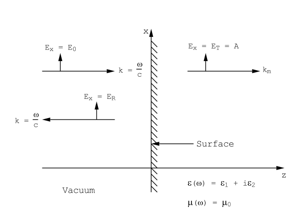
The plane wave propagating in the material (z > 0) must have the same frequency as the incident wave because the response of the material is driven by the incident electric field at the circular frequency ω. However, its wavevector need not be the same as for free space; it must be chosen so as to satisfy Maxwell’s equations. The amplitude of the wave in the material must be chosen so as to satisfy boundary conditions on the surface of discontinuity between the material and vacuum at z=0.

In the material (z > 0) Maxwell’s equations can be written

\[\operatorname{curl}(\vec{\text{E}})=i \omega \mu_{0} \vec{\text{H}}. \label{10.3}\]

It is assumed that there is no free current density, \(\vec{J}_{\text{f}}=0\), so that \(\operatorname{curl}(\vec{\text{H}})\) simplifies to

\[\operatorname{curl}(\vec{\text{H}})=-i \omega \vec{\text{D}}=-i \omega \epsilon_{\text{r}} \epsilon_{0} \vec{\text{E}}. \label{10.4}\]

It is also assumed that there is no free charge density in the material so that

\[\operatorname{div}(\vec{\text{D}})=0 . \label{10.5}\]

In the material we assume that \(\vec{\text{B}}=\mu_{0} \vec{\text{H}}\) and therefore

\[\operatorname{div}(\vec{\text{H}})=0. \label{10.6}\]

In writing these equations use has been made of the definitions from linear response theory in which it is assumed that the polarization per unit volume is a linear function of the electric field strength:

\[\vec{\text{P}}(\omega)=\epsilon_{0} \chi_{\text{E}}(\omega) \vec{\text{E}}, \nonumber \]

and

\[\vec{\text{D}}=\epsilon_{0} \vec{\text{E}}+\vec{\text{P}} , \nonumber \]

so that

\[\vec{\text{D}}=\left[1+\chi_{\text{E}}(\omega)\right] \epsilon_{0} \vec{\text{E}}=\epsilon_{\text{r}} \epsilon_{0} \vec{\text{E}} . \label{10.7}\]

The relative dielectric function \(\epsilon_{\text{r}}(\omega)\) will, in general, be a complex number because the response of the material, \(\vec P\), to a driving electric field, \(\vec E\), is not in phase with the electric field. In the above equations the time dependence of the fields, exp (−iωt) , has been explicitly used. The divergence of \(\vec D\) is zero because it has been explicitly assumed that the material is uncharged. If the electric field is taken to have only an x-component, and to be propagating along z as shown in Figure (10.1.1), then its curl simplifies to give (from Equation (\ref{10.3})

\[\frac{\partial \text{E}_{\text{x}}}{\partial \text{z}}=i \omega \mu_{0} \text{H}_{\text{y}} ; \label{10.8}\]

it follows from this that the magnetic field has only a y-component. Similarly from Equation (\ref{10.4}) one finds

\[\frac{\partial \text{H}_{\text{y}}}{\partial \text{z}}=i \omega \epsilon_{\text{r}} \epsilon_{0} \text{E}_{\text{x}} . \label{10.9}\]

Both \(\vec E\) and \(\vec H\) in the plane wave of Equation (\ref{10.2}) automatically satisfy the condition that their divergences are zero because they are transverse waves; thus Equations (\ref{10.5}) and (\ref{10.6}) are satisfied. From Equations (\ref{10.8}) and (\ref{10.9}) one can obtain

\[\frac{\partial^{2} \text{E}_{\text{x}}}{\partial^{2} \text{z}}=-\epsilon_{\text{r}} \epsilon_{0} \mu_{0} \omega^{2} \text{E}_{\text{x}}=-\epsilon_{\text{r}}\left(\frac{\omega}{\text{c}}\right)^{2} \text{E}_{\text{x}} . \label{10.10}\]

It follows that a wave in the material will satisfy Maxwell’s equations providing that

\[\text{k}_{\text{m}}^{2}=\epsilon_{\text{r}}\left(\frac{\omega}{\text{c}}\right)^{2} . \label{10.11}\]

This means that there are two waves in the material that can be used to satisfy Maxwell’s equations:

\[\text{k}_{\text{m}}=+\left(\frac{\omega}{\text{c}}\right) \sqrt{\epsilon_{\text{r}}}=\left(\frac{\omega}{\text{c}}\right)(\text{n}+i \kappa) , \label{10.12}\]

and

\[ \text{k}_{\text{m}}=-\left(\frac{\omega}{\text{c}}\right) \sqrt{\epsilon_{\text{r}}}=-\left(\frac{\omega}{\text{c}}\right)(\text{n}+i \kappa), \label{10.13}\]

where

\[\epsilon_{\text{r}}=(\text{n}+i \kappa)^{2}=\left(\text{n}^{2}-\kappa^{2}\right)+2 i \text{n} \kappa , \label{10.14}\]

and n and κ are defined by Equation (\ref{10.14}).

If the parameter κ is greater than zero the wave-vector (\ref{10.12}) represents a wave whose amplitude decays to the right since the constant A in Equation (\ref{10.2}) is multiplied by the factor

\[\exp \left(-\left(\frac{\omega}{\text{c}}\right) \kappa \text{z}\right) . \nonumber \]

On the other hand, the wave-vector (\ref{10.13}) represents a wave whose amplitude increases to the right in proportion to

\[\exp \left(+\left(\frac{\omega}{\text{c}}\right) \kappa \text{z}\right) . \nonumber \]

This wave which grows towards the interior of the material clearly cannot be appropriate for the present problem because it would imply that the wave was being amplified by its passage through the passive medium in the right half-space of Figure (10.1.1). It can be concluded that the wave in the material for z≥0 must have the form

\[\text{E}_{\text{x}}=\text{A} \exp \left(-\left(\frac{\omega}{\text{c}}\right) \kappa \text{z}\right) \exp \left(i\left(\frac{\text{n} \omega}{\text{c}} \text{z}-\omega \text{t}\right)\right) , \label{10.15}\]

and from either of equations (\ref{10.8}) or (\ref{10.9})

\[\text{H}_{\text{y}}=\sqrt{\frac{\epsilon_{0}}{\mu_{0}}}(\text{n}+i \kappa) \text{A} \exp \left(-\left(\frac{\omega}{\text{c}}\right) \kappa \text{z}\right) \exp \left(i\left(\frac{\text{n} \omega}{\text{c}} \text{z}-\omega \text{t}\right)\right) . \label{10.16}\]

Notice that the ratio of H_y to E_x is different from the vacuum case:

\[\frac{\text{H}_{\text{y}}}{\text{E}_{\text{x}}}=(\text{n}+i \kappa) \sqrt{\frac{\epsilon_{0}}{\mu_{0}}} , \label{10.17}\]

as opposed to

\[\frac{\text{H}_{\text{y}}}{\text{E}_{\text{x}}}=\sqrt{\frac{\epsilon_{0}}{\mu_{0}}}=\frac{1}{137} \quad O h m^{-1} \nonumber \]

for free space.

The average energy density stored in the electric field is given by

\[\text{W}_{\text{E}}=\frac{\vec{\text{E}} \cdot \vec{\text{D}}}{2} \nonumber \]

from Poynting’s Theorem and the fact that \(\vec D\) is proportional to \(\vec E\), see Chapter(8). The average energy density stored in the electric field is given by

\[<\text{W}_{\text{E}}>=\frac{1}{4} \operatorname{Real}\left(\vec{\text{E}} \cdot \vec{\text{D}}^{*}\right)=\frac{1}{4} \operatorname{Real}\left(\epsilon_{\text{r}} \epsilon_{0} \text{E}^{2}\right) \nonumber \]

or

\[<\text{W}_{\text{E}}>=\frac{1}{4} \epsilon_{0}\left(\text{n}^{2}-\kappa^{2}\right)|\text{A}|^{2} \exp \left(-\left(\frac{2 \omega}{\text{c}}\right) \kappa \text{z}\right) \quad \text { Joules } / m^{3} . \label{10.18}\]

The average energy density stored in the magnetic field is given by

\[\begin{align}
<\text{W}_{\text{B}}>&=\frac{\mu_{0}}{4} \operatorname{Real}\left(\text{HH}^{*}\right) \\
&=\frac{\epsilon_{0}}{4}\left(\text{n}^{2}+\kappa^{2}\right)|\text{A}|^{2} \exp \left(-\left(\frac{2 \omega}{\text{c}}\right) \kappa \text{z}\right) \quad \text { Joules} / m^{3} \nonumber
\end{align} \]

The sum of these two energy densities is

\[<\text{W}>=<\text{W}_{\text{E}}>+<\text{W}_{\text{B}}>=\frac{\epsilon_{0} \text{n}^{2}}{2} \quad|\text{A}|^{2} \exp \left(-\left(\frac{2 \omega}{\text{c}}\right) \kappa \text{z}\right) \quad \text { Joules} / m^{3} . \label{10.20}\]

The energy density decays towards the interior of the material as one would expect.

The Poynting vector, \(\vec{\text{S}}=\vec{\text{E}} \times \vec{\text{H}}\), has only a z-component

\[\begin{align}
<\text{S}_{\text{z}}>&=\frac{1}{2} \operatorname{Real}\left(\text{E}_{\text{x}} \text{H}_{\text{y}}^{*}\right) \\
&=\frac{\text{n}}{2} \sqrt{\frac{\epsilon_{0}}{\mu_{0}}}|\text{A}|^{2} \exp \left(-\left(\frac{2 \omega}{\text{c}}\right) \kappa \text{z}\right) \quad \text {Watts } / m^{2} \nonumber
\end{align}\]

or

\[<\text{S}_{\text{z}}>=\frac{\text{c}}{\text{n}}<\text{W}>\quad \text { Watts } / \text{m}^{2} . \label{10.22}\]

The energy flow in the wave takes place with the velocity c/n. The number n is called the index of refraction. Under some circumstances the index of refraction may be less than 1. In that case the phase velocity in the material exceeds the velocity of light in vacuum. It appears at first sight that a phase velocity greater than the speed of light in vacuum must violate one of the postulates of the theory of relativity. However, no information can be transmitted using a wave of constant amplitude stretching over all time from t=-∞ to t=∞. In order to transmit a message one must modulate the amplitude, or the frequency, of the wave. Any such modulation is propagated with the group velocity; it can be shown that the group velocity is always less than the speed of light in vacuum.

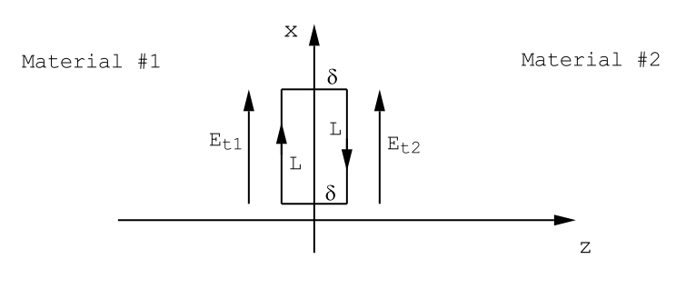
Having determined the wave-vector of the disturbance generated in the material filled half-space by the incident electromagnetic wave, it remains to calculate the amplitude of this disturbance at z=0. In order to find the amplitude A it is necessary to apply appropriate boundary conditions on E_x and H_y on the interface plane z=0.

Figure \(\PageIndex{2}\): The Maxwell equation \(\operatorname{curl}(\vec{\text{E}})=-\partial \vec{\text{B}} / \partial \text{t}\) requires the tangential components of \(\vec E\) to be continuous across any interface. See the text.