11.2: Strip-lines

See Figure (11.1.2). The electric field has only an x-component, if edge effects are neglected, and in the first approximation this component is independent of position across the width of the strip, i.e. E_x is independent of y. Similarly, the magnetic field has only a y-component and this is independent of x and y. From the Maxwell equation

\[\operatorname{curl}(\vec{\text{E}})=-\frac{\partial \vec{\text{B}}}{\partial \text{t}}=-\mu_{0} \frac{\partial \vec{\text{H}}}{\partial \text{t}}\nonumber \]

one has

\[\frac{\partial \text{E}_{\text{x}}}{\partial \text{z}}=-\mu_{0} \frac{\partial \text{H}_{\text{y}}}{\partial \text{t}}. \label{11.1}\]

From the Maxwell equation

\[\operatorname{curl}(\vec{\text{H}})=\frac{\partial \vec{\text{D}}}{\partial \text{t}}=\epsilon_{0} \frac{\partial \vec{\text{E}}}{\partial \text{t}}\nonumber \]

one finds

\[-\frac{\partial \text{H}_{\text{y}}}{\partial \text{z}}=\epsilon_{0} \frac{\partial \text{E}_{\text{x}}}{\partial \text{t}}. \label{11.2}\]

Equations (\ref{11.1}) and (\ref{11.2}) can be combined to obtain

\[\begin{align}
&\left(\frac{\partial^{2} \text{E}_{\text{x}}}{\partial \text{z}^{2}}\right)=-\mu_{0}\left(\frac{\partial^{2} \text{H}_{\text{y}}}{\partial \text{z} \partial \text{t}}\right)=\epsilon_{0} \mu_{0}\left(\frac{\partial^{2} \text{E}_{\text{x}}}{\partial \text{t}^{2}}\right), \label{11.3}\\
&\left(\frac{\partial^{2} \text{H}_{\text{y}}}{\partial \text{z}^{2}}\right)=-\epsilon_{0}\left(\frac{\partial^{2} \text{E}_{\text{x}}}{\partial \text{z} \partial \text{t}}\right)=\epsilon_{0} \mu_{0}\left(\frac{\partial^{2} \text{H}_{\text{y}}}{\partial \text{t}^{2}}\right). \nonumber
\end{align}\]

The first of equations (\ref{11.3}) can be satisfied by any function of the form

\[\text{E}_{\text{x}}(\text{z}, \text{t})=\text{F}(\text{z}-\text{ct})+\text{G}(\text{z}+\text{ct}), \label{11.4}\]

where \(\text{c}=1 / \sqrt{\epsilon_{0} \mu_{0}}\) is the speed of light. This statement can be checked by carrying out the differentiations of Equations (\ref{11.3}):

\[\frac{\partial \text{E}_{\text{x}}}{\partial \text{z}}=\frac{\partial \text{F}}{\partial \text{z}}+\frac{\partial \text{G}}{\partial \text{z}}, \quad \frac{\partial \text{E}_{\text{x}}}{\partial \text{t}}=-\text{c} \frac{\partial \text{F}}{\partial \text{z}}+\text{c} \frac{\partial \text{G}}{\partial \text{z}} \nonumber \]

and

\[\frac{\partial^{2} \text{E}_{\text{x}}}{\partial \text{z}^{2}}=\frac{\partial^{2} \text{F}}{\partial \text{z}^{2}}+\frac{\partial^{2} \text{G}}{\partial \text{z}^{2}}, \quad \frac{\partial^{2} \text{E}_{\text{x}}}{\partial \text{t}^{2}}=\text{c}^{2} \frac{\partial^{2} \text{F}}{\partial \text{z}^{2}}+\text{c}^{2} \frac{\partial^{2} \text{G}}{\partial \text{z}^{2}}. \nonumber\]

Therefore indeed one finds that

\[\frac{\partial^{2} \text{E}_{\text{x}}}{\partial \text{z}^{2}}=\frac{1}{\text{c}^{2}} \frac{\partial^{2} \text{E}_{\text{x}}}{\partial \text{t}^{2}}=\epsilon_{0} \mu_{0} \frac{\partial^{2} \text{E}_{\text{x}}}{\partial \text{t}^{2}}, \nonumber \]

for any arbitrary functions F,G! This means that pulses having any time variation can be transmitted down the line with no distortion. In the real world the pulses do become distorted as a consequence of frequency dependent losses in the line, but for the time being we have only to do with ideal systems that are composed of perfect conductors and lossless dielectrics and such ideal systems transmit pulses without attenuation and with no distortion. The electric field E_x = F(z − ct) corresponds to a pulse propagating along the strip-line in the positive z-direction with the speed of light c. The magnetic field associated with this electric field pulse can be obtained from Equation (\ref{11.1}) or (\ref{11.2}):

\[\frac{\partial \text{H}_{\text{y}}}{\partial \text{z}}=-\epsilon_{0} \frac{\partial \text{E}_{\text{x}}}{\partial \text{t}}=\epsilon_{0} \text{c} \frac{\partial \text{F}}{\partial \text{z}}, \nonumber \]

therefore

\[\text{H}_{\text{y}}=\epsilon_{0} \text{c} \text{F}(\text{z}-\text{ct})=\frac{1}{\text{Z}_{0}} \text{F}(\text{z}-\text{ct}). \nonumber\]

In other words, H_y = E_x/Z₀, where Z₀ = 1/(c\(\epsilon_{0}\))=377 Ohms, the impedance of free space.

The electric field E_x = G(z + ct) corresponds to a pulse propagating in the negative z-direction with the speed of light c. The corresponding magnetic field pulse is given by

\[\frac{\partial \text{H}_{\text{y}}}{\partial \text{z}}=-\epsilon_{0} \frac{\partial \text{E}_{\text{x}}}{\partial \text{t}}=-\epsilon_{0} \text{c} \frac{\partial \text{G}}{\partial \text{z}}, \nonumber \]

or

\[\text{H}_{\text{y}}=-\epsilon_{0} \text{c} \text{G}(\text{z}+\text{ct})=-\text{E}_{\text{x}} / \text{Z}_{0}. \nonumber \]

Note that the sign of the magnetic field component is opposite for the forward propagating and the backwards propagating pulses.

Figure \(\PageIndex{3}\): Cross-section through a co-axial cable. The electric field has a radial component, E_r , and the magnetic field has only the component H_θ independent of the angle θ.

It is usually more convenient to describe pulses on a strip-line or on a coaxial cable in terms of voltages and currents rather than in terms of electric and magnetic fields. The potential difference between the two conducting planes in the strip-line is V = E_xd, where d is the separation between the planes, Figure (11.1.2). On the other hand, surface currents must flow on the perfectly conducting metal planes in order to reduce the magnetic and electric fields to zero inside the metal. This surface current density can be calculated by the application of Stoke’ Theorem to the Maxwell equation

\[\operatorname{curl}(\vec{\text{H}})=\vec{\text{J}}_{f}+\frac{\partial \vec{\text{D}}}{\partial \text{t}} \nonumber \]

for a small loop that spans the metal surface, as shown in Figure (11.2.4).

Figure \(\PageIndex{4}\): A diagrammatic representation of a strip-line in order to illustrate the relation between the electric field, E_x and the potential difference between the two conductors, and to illustrate the connection between the magnetic field, H_y and the surface current density. The potential difference is V=E₀d, and the bottom conductor is positive with respect to the upper conductor for the fields shown in the figure. The bottom conductor carries a total current I=J_zw=H₀w Amps.

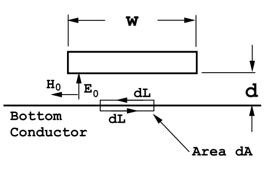
In the limit as the area of the loop, dA, shrinks to zero the term ∂\(\vec D\) /∂t gives nothing so that

\[\int \int_{A r e a} \text{d} \text{S} \operatorname{curl}(\vec{\text{H}}) \cdot \hat{u}_{n}=\oint_{C} \vec{\text{H}} \cdot \vec{\text{d} \vec{\text{L}}}=\text{J}_{2} \text{d} \text{L}, \nonumber \]

where J_z is the surface current density and \(\hat{u}_{n}\) is a unit vector perpendicular to dA. Therefore

\[\text{H}_{0} \text{dL}=\text{J}_{\text{z}} \text{dL} \nonumber \]

so that

\[\text{J}_{\text{z}}=\text{H}_{0}. \nonumber\]

This current density flows along +z in the bottom conductor. The total current carried by the bottom conductor is just proportional to the width of the active region on the strip-line:

\[\text{I}=\text{J}_{\text{z}} \text{w}=\text{H}_{0} \text{w} \quad \text { Amps. }. \nonumber \]

The potential difference between the two conductors is

\[\text{V}=\text{E}_{0} \text{d} \quad \text { Volts }, \nonumber \]

and the bottom plane is positive with respect to the upper plane for the fields shown in the figure.

The characteristic impedance of the line, Z₀ = V/I Ohms, is given by

\[\text{Z}_{0}=\frac{\text{E}_{0} \text{d}}{\text{H}_{0} \text{w}}=\frac{\text{d}}{\text{w}} \sqrt{\mu_{0} / \epsilon_{0}}, \label{11.5}\]

because for a forward propagating wave

\[\text{H}_{0}=\epsilon_{0} \text{c} \text{E}_{0}=\sqrt{\epsilon_{0} / \mu_{0}} \text{E}_{0}. \nonumber \]

The conductors in a practical strip-line are usually separated by a nonmagnetic and non-conducting dielectric material characterized by a magnetic permeability µ₀ and a dielectric constant \(\epsilon\). The above equations are still applicable to such a strip-line providing that dielectric losses can be neglected: one has only to replace \(\epsilon_{0}\) by \(\epsilon\).

In terms of potential difference and current, the picture that emerges is the one illustrated in Figure (11.2.5). A voltage pulse of arbitrary shape propagates along the line with a velocity v that is determined by the properties of the dielectric spacer (here assumed to be lossless). For a non-magnetic spacer material having a dielectric constant \(\epsilon\) this velocity is given by

\[\text{v}=\frac{1}{\sqrt{\epsilon \mu_{0}}}. \label{11.6}\]

The voltage pulse is accompanied by a current pulse of the same shape as the voltage pulse. The scaling factor between current and voltage is the characteristic impedance of the line. The characteristic impedance depends upon the strip-line geometry:for the plane strip-line of Figure (11.2.4) it is given by

\[\text{Z}_{0}=\frac{\text{d}}{\text{w}} \sqrt{\frac{\mu_{0}}{\epsilon}}=\frac{\text{d}}{\text{w}} \frac{1}{\epsilon \text{v}}. \label{11.7}\]

Figure \(\PageIndex{5}\): Voltage and current pulses on a transmission line.

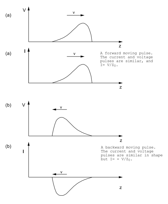
For a forward moving pulse

\[\text{V}=+\text{Z}_{0} \text{I}, \label{11.8}\]

and for a backward moving pulse

\[ \text{V}=-\text{Z}_{0} \text{I},\label{11.9}\]

where V is the potential difference in Volts and I is the current on the transmission line in Amps.

Maxwell’s equations, (\ref{11.3}), can be rewritten in terms of the potential difference, V, and the current on the line, I. Since E_x is proportional to V the first of equations (\ref{11.3}) becomes

\[\frac{\partial^{2} \text{V}}{\partial \text{z}^{2}}=\frac{1}{\text{v}^{2}} \frac{\partial^{2} \text{V}}{\partial \text{t}^{2}}. \label{11.10}\]

Similarly, since H_y is proportional to the current I, the second of equations(11.3) becomes

\[\frac{\partial^{2} I}{\partial z^{2}}=\frac{1}{v^{2}} \frac{\partial^{2} I}{\partial t^{2}}. \label{11.11}\]

These telegraph line equations were derived by Lord Kelvin in 1855 (this was before Maxwell’s equations had been discovered) by treating the transmission line as a repeating series of inductances shunted by capacitors. See Electromagnetic Theory by J.A.Stratton, McGraw-Hill, New York, 1941, section 9.20, Figure (103); for a lossless line R=0 and G=∞.