13.8: Chapter 8

Problem (8.1)

A long straight non-magnetic wire carries a steady current of I Amps. The resistance of the wire is R Ohms/meter. Use Poynting's theorem to show that the energy flow into the wire is I²R/meter.

Answer (8.1)

At the surface of the wire the magnetic field is tangential. From CurlB = µ_oJ_f (No M, no time variation) one has, using Stokes' theorem,

\[2 \pi \mathrm{aB}_{\theta}=\mu_{0} I\nonumber\]

So \(\text{B}_{\theta}=\frac{\mu_{0} I}{2 \pi_{2}} \) or \(\text{H}_{\theta}=\frac{\text{I}}{2 \pi \text{a}} \).

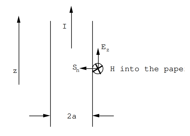
The electric field is also tangential E_z = IR Volts/m.

∴ S = E x H is normal to the wire surface and \(\text{S}_{\text{n}}=\frac{\text{I}^{2} \text{R}}{2 \pi \text{a}}\). Energy flow/m = (S_n)(2\(\pi\)a) = I²R Watts/m.

Problem (8.2).

One meter of wire is bent into a circular form to make a magnetic dipole antenna. The wire carries a current I(t) = I_o sin ωt where I_o = 2 Amps, ω = 2\(\pi\)f, and f = 50 MHz. At what rate does this loop radiate energy?

Answer (8.2).

For a magnetic dipole at the origin, m_z, one has

\(B_{r}=\left(\frac{\mu_{0}}{4 \pi}\right) 2 \cos \theta\left[\frac{m_{z}}{R^{3}}+\frac{\dot{m}_{z}}{c R^{2}}\right]\)

\(\text{B}_{\theta}=\frac{\mu_{0}}{4 \pi} \sin \theta\left[\frac{\text{m}_{\text{z}}}{\text{R}^{3}}+\frac{\dot{\text{m}}_{\text{z}}}{\text{CR}^{2}}+\frac{\ddot{\text{m}_{\text{z}}}}{\text{c}^{2} \text{R}}\right]\)

\(E_{\phi}=-c B_{\theta}=-\left(\frac{\mu_{0}}{4 \pi}\right) \operatorname{csin} \theta\left[\frac{\dot{m}_{z}}{c R^{2}}+\frac{\ddot{m}_{z}}{c^{2} R}\right]\)

(part of B_θ that is proportional to the time derivatives).

Very far from the magnetic dipole one has only the radiation field terms ~ 1/R:

\(E_{\phi}=-\left(\frac{\mu_{0}}{4 \pi}\right) \quad \sin \theta \frac{\ddot{m}_{z}}{C R}\)

\(\text{B}_{\theta}=\left(\frac{\mu_{0}}{4 \pi}\right) \sin \theta \frac{\ddot{\text{m}}_{\text{z}}}{\text{c}^{2} \text{R}}\)

or \(\text{H}_{\theta}=\frac{1}{4 \pi} \sin \theta \frac{\ddot{\text{m}}_{\text{z}}}{\text{c}^{2} \text{R}}\)

S = E x H has only a radial component

\(S_{r}=\frac{\mu_{0}}{(4 \pi)^{2}} \sin ^{2} \theta \frac{\left(\ddot{m}_{z}\right)^{2}}{c^{3} R^{2}}\).

If I = I_o sinωt then m_z = (\(\pi\)a2) I_o sinωt

\[\ddot{m}_{z}=-\omega^{2} \quad\left(\pi \text{a}^{2} I_{0}\right) \quad \sin \omega t.\nonumber\]

Let m_o = \(\pi\)a²Io. In this problem 2\(\pi\)a = 1 m so m_o = 0.159 Amp m².

At R and at the angle θ the time averaged Poynting vector is given by

\(\left\langle S_{r}\right\rangle=\frac{\mu_{0}}{(4 \pi)^{2}} \sin ^{2} \theta \frac{\omega^{4} m_{0}^{2}}{2 c^{3} R^{2}}=0.0363 \frac{\sin ^{2} \theta}{R^{2}} \quad \text { Watts } / m^{2}\)

Integrate this over a sphere of radius R. The element of surface area is dA = 2\(\pi\)R² sin θ dθ

∴ radiated power \(P=(0.0363)(2 \pi) \int_{0}^{\pi} \sin ^{3} \theta d \theta \quad \text { Watts }\)

but \(\int_{0}^{\pi} \sin ^{3} \theta d \theta=4 / 3\)

∴ P = 0.305 Watts

Problem (8.3)

An electric dipole whose strength is p₀= 10^-7 Coulomb-meters oscillates at a frequency f= 50 MHz. Let the dipole be oriented along z.

(a) Estimate the electric field amplitude measured by an observer on the x-axis at a mean distance of 5 meters from the dipole. Compare the near field terms with the far-field, or radiation term. Note that the \(\dot{p}\) term is in quadrature with the other two terms so that it contributes only about 2% to the electric field amplitude.

(b) How big is the phase shift between the time variation of the dipole and the electric field measured by the observer?

(c) What intensity would the observer measure at the coordinates (5,0,0); i.e. what is the value of <S_x> )?

(d) What would be the intensity of the radiation measured by an observer on the z-axis 5 meters from the oscillating dipole?

(e) At what total rate does this dipole radiate energy?

(f) This dipole can be modelled by two spheres each having a radius of 0.1 meters and separated by 0.5 meters center to center. One sphere carries an initial charge of Q= +2x10^-7 Coulombs, the other sphere carries an initial charge of -2x10^-7 Coulombs. The two spheres are suddenly connected by a conducting wire and the two charges oscillate back and forth. Estimate how long is required for this system to radiate away e^-1 of its initial energy. ( The stored energy is proportional to Q²; the rate at which energy is radiated away is proportional to Q² because p_z= Qd. It follows that the energy stored on the two spheres will decay exponentially in time).

Answer (8.3).

(a) p_z = p₀ e^-iωt

where ω= 2\(\pi\)f= 3.14x10⁸ radians/sec, and \(\frac{\omega}{c}=1.047 \text{m}^{-1}\).

\[\text{E}_{\text{r}}=\frac{1}{4 \pi \varepsilon_{0}} 2 \cos \theta\left(\frac{\text{p}_{z}}{\text{R}^{3}}+\frac{\dot{\text{p}_{z}}}{\text{cR}^{2}}\right)\nonumber\]

\[\text{E}_{\theta}=\frac{1}{4 \pi \varepsilon_{0}} \sin \theta\left(\frac{\text{p}_{z}}{\text{R}^{3}}+\frac{\dot{\text{p}_{\text{z}}}}{\text{cR}^{2}}+\frac{\ddot{\text{p}_{\text{z}}}}{\text{c}^{2} \text{R}}\right)\nonumber\]

\[\text{E}_{\phi}=0\nonumber\]

\[\text{cB}_{\phi}=\frac{1}{4 \pi \varepsilon_{0}} \sin \theta\left(\frac{\dot{\text{p}}_{\text{z}}}{\text{cR}^{2}}+\frac{\ddot{\text{p}_{\text{z}}}}{\text{c}^{2} \text{R}}\right)\nonumber\]

\[\text{B}_{\text{r}}=\text{B}_{\theta}=0.\nonumber\]

On the x-axis θ= \(\pi\)/2, and Cosθ=0, Sinθ=1. Consequently, one has only to worry about the electric field component, E_θ. Taking out the common factors one has

first term: \(\frac{1}{R^{3}}=\frac{1}{125}=0.008\)

second term: \(-\frac{i \omega}{c R^{2}}=-0.042 i\)

third term: \(\frac{-\omega^{2}}{c^{2} R}=-0.219\)

The total field is proportional to -0.211 - 0.042i. The quadrature term makes only a ~ 2% correction to the field. For an observer along x and 5 meters from the dipole the electric field is polarized along z: it is given by

\[\left|\mathrm{E}_{\mathrm{z}}\right|=193 \text { Volts/meter. }\nonumber\]

(b) The phase shift between the time variation of the dipole and the electric field at the observer is

\[\Delta \phi=\frac{\omega R}{c}=5.235 \text { radians }=300^{\circ}\nonumber\]

(c) For an observer at (5,0,0)

\[\text{E}_{\theta}=-90(2.11+0.419 \text{i})\nonumber\]

\[\text{H}_{\phi}=-0.2387(2.193+0.419 \text{i})\nonumber\]

Therefore

\(\left\langle S_{X}\right\rangle=\frac{1}{2} \operatorname{Real}\left(E_{\theta} H_{\phi}^{\star}\right)=10.74(4.627+0.176+0.035 i) \quad \text { Watts } / m^{2}\),

\(\left\langle S_{X}\right\rangle=51.6 \text { Watts } / m^{2}\)

(d) For an observer at (0,0,5) the angle θ is zero, and consequently E_θ=0 and B_\(\phi\)= H_\(\phi\)= 0; thus <S_z>= 0.

(e) \(\langle\text{P}\rangle=\frac{1}{3} \frac{\text{C}}{4 \pi \varepsilon_{0}} \text{p}_{0}^{2}\left(\frac{\omega}{\text{c}}\right)^{4}=10.8 \text{kWatts}\)

Problem (8.4)

A 10 turn circular coil of wire is centered on the origin and the plane of the coil lies parallel with the xy plane. The coil has a mean radius of 5 cm and it carries a current I(t)= I₀Sinωt where I₀= 100 Amps, and ω= 2\(\pi\)f where f= 20 MHz. An observer in the xy plane, and 1 km distant from the coil, measures the emf induced in a piece of straight wire 1 meter long due to the radiation field produced by the oscillating current in the coil.

(a) In what direction should the observer orient the wire in order to obtain the maximum signal?

(b) What maximum receiver power would you expect the observer to measure using a matched receiver? The radiation resistance of a short wire of length L meters (L/\(\lambda\)<<1) is given by \(\text{R}=80 \pi^{2}\left(\frac{\text{L}}{\lambda}\right)\) Ohms.

(c) Calculate the total average rate at which energy is radiated by the oscillating magnetic dipole formed by the coil.

Answer (8.4).

(a) The wire should be oriented parallel with the xy plane and perpendicular to the line joining the observer to the coil. The electric field has only an E_\(\phi\) component.

(b) For this problem one can ignore the near field terms and calculate only the radiation field terms. These are

\[\text{B}_{\theta}=\frac{\mu_{0}}{4 \pi} \sin \theta \frac{\ddot{m}_{z}}{c^{2} R} \quad \text { Teslas },\nonumber\]

\[\text{E}_{\phi}=-\text{cB}_{\theta} \text { Volts/meter. }\nonumber\]

In this problem m_z= m₀e^-iωt where m₀= 7.85 Amp-meters², ω= 1.257x10⁸ radians/sec., \(\frac{\omega}{c}=0.419 \text{m}^{-1}\) and \(\lambda\)=15 m. For an observer in the x-y plane the angle θ= \(\pi\)/2 so that

\[\text{B}_{\theta}=-\frac{\mu_{0}}{4 \pi} \frac{\omega^{2}}{\text{c}^{2}} \frac{\text{m}_{0}}{\text{R}}=1.378 \times 10^{-10} \text {Teslas }\nonumber\].

The electric field strength at the observer will be \(\text{E}_{\phi}=-\text{cB} \theta=41.3 \times 10^{-3} \text{Volts} / \text{m}\). The current induced in the wire will have the spatial variation \(I(z)=I_{0} \sin \left(\frac{2 \pi}{\lambda}\left[\frac{L}{2}-z\right]\right)\) for z>0 with a similar variation for z<0. The average power delivered to the antenna will be

\(<P_{i}>=\frac{1}{2} (2) E_{0} I_{0} \int_{0}^{L} d z \sin \left(\frac{2 \pi}{\lambda}\left[\frac{L}{2}-z\right]\right)=E_{0} I_{0} \frac{\lambda}{2 \pi}\left(1-\cos \left(\frac{\pi L}{\lambda}\right)\right),\)

or for small L/\(\lambda\) \(<\text{P}_{\text{i}}>\cong \operatorname{E}_{0} \text{I}_{0}\left(\frac{\pi}{4}\right)\left(\frac{\text{L}^{2}}{\lambda}\right)\). Half this power is delivered to the load:

\(\text{E}_{0} \text{I}_{0}\left(\frac{\pi}{4}\right)\left(\frac{\text{L}^{2}}{\lambda}\right)=\text{I}_{0}^{2} \text{R}\), where \(\text{R}=20 \pi^{2}\left(\frac{\text{L}}{\lambda}\right)^{2}=0.877 \quad \text{Ohms} .\)

I₀ = 2.468x10^-3 Amps. The power delivered to the matched load is \(<\text{P}_{\text{L}}>=\frac{\text{R}}{2} \text{I}_{0}^{2}=2.67 \times 10^{-6} \text{Watt} \text{s}\).

(c) The total rate at which a magnetic dipole radiates energy is given by

\[P_{M}=\frac{c}{3} \frac{\mu_{0}}{4 \pi}\left(\frac{\omega}{c}\right)^{4} m_{0}^{2} \text { Watts }=19.0 \text { Watts. }\nonumber\]

This contributes an amount Z Ohms to the coil resistance where \(\frac{I_{0}^{2} z}{2}=19.0 \text { Watts }\). This gives Z= 3.8x10^-3 Ohms since the current amplitude was assumed to be 100 Amps. This means that very heavy wire should be used for the oscillator tank coil if one wishes most of the input power to be radiated as electromagnetic energy rather than dissipated in the coil as heat.

Problem (8.5).

Two identical electric dipoles are driven by the same oscillator at a frequency of 20 MHz but there is a phase shift of β radians between them. The dipoles are both oriented along the z-axis, but one dipole is located at (5,0,0), the other is located at (-5,0,0). Describe the angular variation of the maximum radiation field intensity produced by these two dipoles as measured by an observer confined to the x-y plane and located a constant distance of 1 km from the origin; i.e. make a plot of the time-averaged Poynting vector as a function of the angle \(\phi\) measured from the x-axis for (a) β=0 radians, and (b) \(\beta=\frac{\pi}{2}\) radians.

Answer (8.5).

One has only to worry about the far field terms generated by the oscillating dipoles, however the phase at the observer is very important in this problem.

Dipole #1: \[\text{E}_{\text{z}}^{1}=\frac{1}{4 \pi \varepsilon_{0}}\left(\frac{\omega}{\text{c}}\right)^{2} \frac{\text{p}_{0}}{\text{R}} \text{e}^{-\text{i} \omega\left(\text{t}-\left[\frac{\text{R}-\text{d} \cos \phi}{\text{c}}\right]\right)} \exp (\text{i} \beta)\nonumber\]

Dipole #2: \[\text{E}_{\text{z}}^{1}=\frac{1}{4 \pi \varepsilon_{0}}\left(\frac{\omega}{\text{c}}\right)^{2} \frac{\text{p}_{0}}{\text{R}} e^{-\text{i} \omega\left(\text{t}-\left[\frac{\text{R}+\text{d} \cos \phi}{\text{c}}\right]\right)}. \nonumber\]

In writing these expressions explicit account has been taken of the fact that the distance from the observer to each dipole is slightly different. But slight as it may be compared with R, the difference in distance is a large fraction of a wavelength (\(\lambda\)= 15 meters). The total electric field measured by the observer in the x-y plane is given by

\[\text{E}_{\text{z}}=\frac{1}{4 \pi \varepsilon_{0}}\left(\frac{\omega}{\text{c}}\right)^{2} \frac{\text{p}_{0}}{\text{R}} e^{\text{i} \omega(\text{t}-\text{R} / \text{c})} \text{e}^{\text{i} \beta / 2}\left(e^{i \frac{\omega}{c} d C o s \phi+i \beta / 2}+e^{-i \frac{\omega}{c}} d \cos \phi-i \beta / 2\right), \nonumber\]

or

\[\text{E}_{\text{S}}=2 \text{E}_{0} \text{e}^{\text{i} \omega(\text{t}-\text{R} / \text{c})} \text{e}^{\text{i} \beta / 2} \cos \left(\frac{\omega}{\text{c}} \text{d} \cos \phi+\beta / 2\right),\nonumber\]

where \(\text{E}_{0}=\frac{1}{4 \pi \varepsilon_{0}}\left(\frac{\omega}{\text{c}}\right)^{2} \frac{\text{p}_{0}}{\text{R}}\).

The time averaged Poynting vector is proportional to the square of the electric field strength; for one oscillator \(<\text{S}_{0}>=\frac{\text{E}_{0}^{2}}{2 \text{Z}_{0}}\), where Z₀= 377 Ohms. We may therefore write

\[\langle S\rangle=4<S_{0}>\operatorname{Cos}^{2}\left(\frac{\omega}{c} d \operatorname{Cos} \phi+\beta / 2\right).\nonumber\]

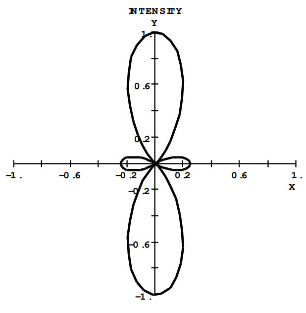
(a) β=0, and d= 5.0 m. (ω/c)= 0.419 cm^-1 so

\[\langle S\rangle=4<S_{0}>\cos ^{2}(2.094 \cos \phi).\nonumber\]

A polar plot of Cos²(2.094Cos\(\phi\)) is shown below.

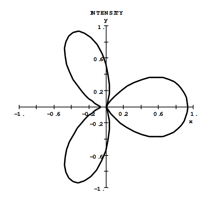
(b) For a phase shift of \(\pi\)/2 between the oscillators one finds

\[\langle S\rangle=4 S_{0} \operatorname{Cos}^{2}\left(\frac{\omega}{c} d \cos \phi+\frac{\pi}{4}\right)=4 S_{0} \cos ^{2}\left(2.094 \cos \phi+\frac{\pi}{4}\right).\nonumber\]

A plot of the \(\cos ^{2}\left(2.094 \cos \phi+\frac{\pi}{4}\right)\) pattern is shown below.

Problem (8.6).

100 Watts/m² of monochromatic laser light having a free space wavelength of \(\lambda\)= 0.5145 µm is used to illuminate a stationary hydrogen atom. For this problem atomic hydrogen can be modelled by an oscillator having a single resonant frequency given by the n=1 to n=2 transition at 10.18 eV. the oscillator strength may be taken to be unity

(a) Estimate the total power removed from the incident beam by the hydrogen atom.

(b) How much energy would be scattered per second into a photomultiplier tube having an aperature of 3 cm and located 10 cm from the atom? The axis of the photomultiplier tube is oriented perpendicular to the incident beam in such a direction as to intercept the maximum scattered power.

Answer (8.6).

(a) Calculate the resonant frequency associated with the n=1 to n=2 transition in the hydrogen atom:

\[ \begin{array}{c} 10.18 \text{eV}=16.31 \times 10^{-19} \text {Joules.} \\ \text{hf}_{0}=16.31 \times 10^{-19}, \quad \text {so } \\ \text{f}_{0}=2.461 \times 10^{15} \text{Hz} \text { and } \lambda=0.1219 \mu \text{m.} \\ \omega_{0}=2 \pi \text{f}_{0}=1.546 \times 10^{16} \text { radians/sec. } \end{array}\nonumber\]

The equation of motion for the bound electron in the hydrogen atom can be written

\[m \frac{d^{2} z}{d t^{2}}+k z=-e E_{0} e^{-i \omega t},\nonumber\]

where \(\text{k} / \text{m}=\omega_{0}^{2}\). Under the influence of a driving field at circular frequency ω the electron amplitude is given by

\[z_{0}=-\frac{(e / m) E_{0}}{\left[\omega_{0}^{2}-\omega^{2}\right]}.\nonumber\]

Now calculate the electric field amplitude in the incident beam. The frequency of the incident light is f= c/\(\lambda\)= 5.831x10¹⁴ Hz, and ω= 3.664x10¹⁵ radians/sec. The power in the incident beam is

\[<S>=\frac{E_{0} H_{0}}{2}=\frac{E_{0}^{2}}{2 Z_{0}}=10^{2} W a t t s / m^{2},\nonumber\]

where Z₀= 377 Ohms. From this expression E₀= 275 Volts/m. For this field amplitude the electron amplitude is

z₀ = -2.14x10^-19 meters, corresponding to

an induced dipole moment amplitude p₀ = - ez₀ = 3.43x10^-38 Coulomb-meters. The averaged power radiated by the oscillating atomic electron is

\[P_{E}=\frac{c}{3} \frac{1}{4 \pi \varepsilon_{0}}\left(\frac{\omega}{c}\right)^{4} p_{0}^{2}=23.53 \times 10^{-30} \text {Watts }\nonumber\]

A photon at 0.5145 µm carries an energy of 38.64x10^-20 Joules. The hydrogen atom scatters the equivalent of 6.1x10^-11 photons per second. One would have to wait approximately 3200 years in order to get only 6 photons! ( 1 year= 3.15x10⁷ seconds).

(b) The area of the photomultiplier tube is \(\pi\)r²= 7.07 cm², therefore \(\frac{\text { Area }}{\text{R}^{2}}=\text{d} \Omega=\frac{7.07}{100}=0.0707\) steradians. The power intercepted by the tube will be given by

\[P_{T}=\frac{1}{8 \pi}\left(\frac{c}{4 \pi \varepsilon_{0}}\right)\left(\frac{\omega}{c}\right)^{4} p_{0}^{2} d \Omega, \text { since } \sin \theta=1\nonumber\]

Therefore P_T= 1.99x10^-31 Watts. In order to get one count per second one would need N= 19.5x10¹¹ hydrogen atoms. This corresponds to 7.2x10^-11 liters at NTP or 7.2x10^-8 cc of gas at NTP. Such an experiment would be feasible using 1 mm cubed of gas at NTP (10^-3 cc); the dark count for a good tube is of order 1.0 counts per second at room temperatures.

Problem (8.7).

A very thin plane, uniform, sheet of dipoles is located in the y-z plane. The dipole moments are aligned along the z-axis and they vary in time like e^-iωt . The polarization density for such a sheet can be written

\[\text{P}_{\text{z}}(\text{x}, \text{y}, \text{z}, \text{t})=\text{P}_{0} \delta(\text{x}) \text{e}^{-\text{i} \omega \text{t}}.\nonumber\]

(a) Show that this time-varying polarization density generates a vector potential which can be written in the form

X>0: \(\text{A}_{\text{z}}(\text{X}, \text{Y}, \text{Z}, \text{t})=\frac{\mu_{0} \text{P}_{0} \text{C}}{2} \text{e}^{\text{i}(\text{kX}-\omega \text{t})}\);

X<0: \(\text{A}_{\text{Z}}(\text{X}, \text{Y}, \text{Z}, \text{t})=\frac{\mu_{0} \text{P}_{0} \text{C}}{2} e^{-\text{i}(\text{k} \text{X}+\omega \text{t})}\).

(Hint: one can use the particular solution for the vector potential in terms of the current density. Note also that A cannot depend upon either Y or Z from the symmetry of the problem; this means that one can carry out the calculation for Y=Z=0. You will run into an indeterminate constant upon carrying out the integral; this does not matter because any constant, no matter how large, can be added to the potential without altering the fields calculated from it.)

(b) Use the above vector potential to calculate the scalar potential from the Lorentz condition \(\operatorname{div} \mathbf{A}+\frac{1}{c^{2}} \frac{\partial V}{\partial t}=0\). Use the potentials to calculate the corresponding electric and magnetic fields.

(c) What is the rate at which energy is radiated away from this sheet of dipoles?

Answer (8.7).

The vector potential is generated by the total current density \(\boldsymbol{J}_{\text{tot}}=\mathbf{J}_{\text{f}}+\operatorname{curl} \mathbf{M}+\frac{\partial \mathbf{p}}{\partial \text{t}}\). For this problem the current density is entirely due to the term \(\frac{\partial \mathbf{p}}{\partial t}\); this term has only a zcomponent, so the vector potential which it generates will have only a z-component.

\[J_{z}=\frac{\partial P_{z}}{\partial t}=-i \omega P_{0} \delta(x) e^{-i \omega t},\nonumber \]

therefore

\[\text{A}_{\text{z}}(\text{X}, \text{Y}, \text{Z}, \text{t})=\frac{\mu_{0}}{4 \pi} \int_{\text{Space}} \frac{\text{dxdydz}\left(-\text{i} \omega \text{P}_{0}\right) \delta(\text{x}) e^{-\text{i} \omega(\text{t}-\text{R} / \text{c})}}{\text{R}}\nonumber\]

where

\[R=\left((X-x)^{2}+(Y-y)^{2}+(Z-z)^{2}\right)^{1 / 2}.\nonumber\]

From the plane symmetry the vector potential A_z cannot depend upon the co-ordinates Y,Z; it is convenient to take Y=Z= 0. One can use polar co-ordinates in the plane and write

\[R=\sqrt{r^{2}+X^{2}},\nonumber\]

and dydz= 2\(\pi\)rdr. The integral over x can be carried out with no effort because of the δ-function. One obtains

\[\text{A}_{\text{z}}(\text{X}, \text{t})=\frac{\mu_{0}}{4 \pi}\left(-\text{i} \omega \text{P}_{0}\right) \int_{0}^{\infty} \frac{2 \pi \text{rdre}^{-\text{i} \omega \text{t}} \text{e}^{\text{i} \frac{\omega \sqrt{\text{r}^{2}+\text{X}^{2}}}{\text{c}}}}{\sqrt{\text{r}^{2}+\text{X}^{2}}}.\nonumber\]

The integral can be carried out with the help of the substitutions

\(u=\sqrt{r^{2}+X^{2}}\) and udu = rdr.

\[\text{A}_{\text{z}}(\text{X}, \text{t})=-\frac{\text{i} \omega \mu_{0} \text{P}_{0}}{2} \text{e}^{-\text{i} \omega \text{t}} \int_{|\text{X}|}^{\infty} \text{du} \text{e}^{\text{i} \omega \text{u} / \text{c}}.\nonumber\]

The constant is ill-defined; ignore it because a constant has no effect on the fields calculated from the vector potential.

\(\text{A}_{\text{z}}(\text{X}, \text{t})=\left(\frac{\mu_{0} \text{cP}_{0}}{2}\right) \text{e}^{\text{i}(\text{k}|\text{X}|-\omega \text{t})}\), where k= ω/c.

For X>0 this represents a wave propagating to the right.

For X<0 this represents a wave propagating to the left.

(b) The scalar potential can be calculated from the Lorentz condition

\[\operatorname{div} \mathbf{A}+\frac{1}{c^{2}} \frac{\partial V}{\partial t}=0.\nonumber\]

For this example, divA=0 so that the scalar potential is also zero.

The electric field has only a z-component which is given by \(\text{E}_{\text{z}}=-\frac{\partial \text{A}_{z}}{\partial t}\).

The magnetic field has only a y-component which is given by \(\text{B}_{\text{Y}}=-\frac{\partial \text{A}_{\text{z}}}{\partial \text{X}}\).

For X>0: \(\text{E}_{\text{z}}=\frac{\text{i} \omega \mu_{0} \text{cP}_{0}}{2} e^{\text{i}(\text{kX}-\omega \text{t})} \quad \text{Volts} / \text{m}\)

\[B_{Y}=-\frac{i k \mu_{0} P_{0} c}{2} e^{i(k X-\omega t)}=-\frac{i \omega \mu_{0} P_{0}}{2} e^{i(k X-\omega t)} \quad \text { Teslas }.\nonumber\]

For X<0: \(\text{E}_{\text{z}}=\frac{\text{i} \omega \mu_{0} \text{cP}_{0}}{2} e^{-\text{i}(\text{kX}+\omega \text{t})} \quad \text{Volts} / \text{m}\),

\[B_{Y}=\frac{i k \mu_{0} P_{0} c}{2} e^{-i(k X+\omega t)}=\frac{i \omega \mu_{0} P_{0}}{2} e^{-i(k X+\omega t)} \quad \text { Teslas }.\nonumber\]

(c) The plane sheet of polarization radiates a plane wave in each direction which is shifted in phase by 90° with respect to the polarization sheet. The average rate at which energy is radiated in either direction is

\[<\left|S_{X}\right|>=\frac{C}{8} \mu_{0} \quad \omega^{2} P_{0}^{2} \quad \text { Watts } / m^{2}.\nonumber\]

Problem (8.8).

A very thin plane, uniform, sheet of dipoles is located in the y-z plane. The dipole moments are aligned along the x-axis and they vary in time like e^-iωt . The polarization density for such a sheet can be written

\(P_{X}(X, Y, z, t)=P_{0} \delta(x) e^{-i \omega t}\).

This problem differs from Prob.(8.7) in the orientation of the dipoles. It is still true that A cannot depend upon either Y or Z because of the planar symmetry.

(a) Show that this time-varying polarization density generates a vector potential which can be written in the form

X>0: \(\text{A}_{\text{X}}(\text{X}, \text{Y}, \text{Z}, \text{t})=\frac{\mu_{0} \text{P}_{0} \text{c}}{2} \text{e}^{\text{i}(\text{kX}-\omega \text{t})}\),

X<0: \(\text{A}_{\text{X}}(\text{X}, \text{Y}, \text{Z}, \text{t})=\frac{\mu_{0} \text{P}_{0} \text{c}}{2} e^{-\text{i}(\text{k} \text{X}+\omega \text{t})}\).

(Hint: one can use the particular solution for the vector potential in terms of the current density. You will run into an indeterminate constant upon carrying out the integral; this does not matter because any constant, no matter how large, can be added to the potential without altering the fields calculated from it.)

(b) Show that the electric and magnetic fields corresponding to the above potentials are zero.

Answer (8.8).

This problem can be solved by direct integration after the manner of Problem(8.7). A more elegant and usefull method starts from the differential equation for the vector potential:

\[\nabla^{2} A_{x}-\frac{1}{c^{2}} \frac{\partial A_{x}}{\partial t^{2}}=-\mu_{0} J_{x}=i \omega \mu_{0} \ P_{0} e^{-i \omega t} \delta(x)\nonumber\]

The free space solutions of this differential equation are:

(i) on the right,x>0; \(\text{A}_{\text{X}}=\text{A}_{0} \text{e}^{\text{i}(\text{kx}-\omega \text{t})}\),

(ii) on the left,x<0; \(A_{X}=A_{0} e^{-i(k x+\omega t)},\)

where k= ω/c. These plane waves satisfy the homogeneous wave equation

\[\nabla^{2} A_{X}-\frac{1}{c^{2}} \frac{\partial A_{X}}{\partial t^{2}}=0.\nonumber\]

The amplitudes of the two waves must be the same by symmetry. Near x=0 one requires

\[\frac{\partial^{2} A_{x}}{\partial x^{2}}+\left(\frac{\omega}{c}\right)^{2} A_{x}=i \omega \mu_{0} P_{0} \delta(x).\nonumber\]

Integrate this equation over a vanishingly small interval around x=0, from x=-ε to x=ε. The result is

\[\left.\frac{\partial \mathrm{A}_{\mathrm{x}}}{\partial \mathrm{x}}\right|_{\varepsilon}-\left.\frac{\partial \mathrm{A}_{\mathrm{x}}}{\partial \mathrm{x}}\right|_{-\varepsilon}+\left(\frac{\omega}{\mathrm{c}}\right)^{2} \mathrm{O}(\varepsilon)=\mathrm{i} \omega \mu_{0} \mathrm{P}_{0}.\nonumber\]

\[\left.\lim _{\varepsilon \rightarrow 0} \frac{\partial \text{A}_{\text{x}}}{\partial \text{x}}\right|_{\varepsilon}=\text{i} \text{kA}_{0}\nonumber\]

\[\left.\lim _{\varepsilon \rightarrow 0} \frac{\partial \text{A}_{\text{X}}}{\partial \text{x}}\right|_{-\varepsilon}=-\text{i} \text{kA}_{0},\nonumber\]

and the term of order ε goes to zero in the limit as ε→0. Therefore,

\[2 \text{i} \text{kA}_{0}=\text{i} \omega \mu_{0} \text{P}_{0}\nonumber\]

and

\[\text{A}_{0}=\frac{\mu_{0} \text{cP}_{0}}{2}.\nonumber\]

(b) The scalar potential can be calculated from the Lorentz condition

\[\operatorname{div} \mathbf{A}+\frac{1}{\text{c}^{2}} \frac{\partial \text{V}}{\partial \text{t}}=0.\nonumber\]

Consider the potentials for x>0; the potentials for x<0 can be handled in the same way.

\[\operatorname{div} \mathbf{A}=\frac{\text{i} \omega \mu_{0} \text{P}_{0}}{2} e^{\text{i}(\text{kx}-\omega \text{t})},\nonumber\]

consequently

\[V=\frac{c^{2} \mu_{0} P_{0}}{2} e^{i(k x-\omega t)}=\frac{P_{0}}{2 \varepsilon_{0}} e^{i(k x-\omega t)}.\nonumber\]

\[\mathbf{E}=-\operatorname{grad} V-\frac{\partial \mathbf{A}}{\partial t},\nonumber\]

so that

\[E_{X}=-\frac{i k P_{0}}{2 \varepsilon_{0}} e^{i(k x-\omega t)}+\frac{i \omega \mu_{0} P_{0} c}{2} e^{i(k x-\omega t)}.\nonumber\]

But \(\frac{\text{i} \omega \mu_{0} \text{P}_{0} \text{c}}{2}=\frac{\text{i} \omega \mu_{0} \text{P}_{0} \text{c}^{2}}{2 \text{c}}=\frac{\text{i} \text{k} \text{P}_{0}}{2 \varepsilon_{0}}\)

so that E_x ≡ 0

Furthermore, curlA ≡ 0 so that there is also no magnetic field component.

Problem (8.9).

very thin plane, uniform, sheet of dipoles is located in the y-z plane. The dipole moments are aligned along the x-axis and their time variation can be described by

\[e^{i(q y-\omega t)}.\nonumber\]

The polarization density for such a sheet can be written

\[\text{P}_{\text{X}}(\text{x}, \text{y}, \text{z}, \text{t})=\text{P}_{0} \delta(\text{x}) \text{e}^{\text{i}(\text{qy}-\omega \text{t})}.\nonumber\]

Calculate the electric and magnetic fields generated by this space and time varying polarization density.

Hint: It is very difficult to calculate the vector potential by direct integration of the expression

\[\mathbf{A}(\mathbf{R}, \text{t}) \frac{\mu_{0}}{4 \pi} \int \frac{\left.\text{d} \tau \frac{\partial \mathbf{p}}{\partial \text{t}}\right|_{\text{t}_{\text{R}}}}{|\mathbf{R}-\mathbf{r}|}.\nonumber\]

It is better to work directly with the differential equation

\[\nabla^{2} A_{x}-\frac{1}{c^{2}} \frac{\partial^{2} A_{x}}{\partial t^{2}}=\mu_{0} i \omega P_{0} \delta(x) e^{i(q y-\omega t)}.\nonumber\]

For x>0 let \(\text{A}_{\text{X}}=\text{A}_{0} \text{e}^{\text{i}(\text{kx}+\text{qy}-\omega \text{t})}\)

For x<0 let \(\text{A}_{\text{x}}=\text{A}_{0} \text{e}^{\text{i}(-\text{kx}+\text{qy}-\omega \text{t})}\).

These functions satisfy the homogeneous equation and represent plane waves propagating away from the dipole plane. The left and right propagating plane waves have the same amplitude by symmetry; this can be deduced directly from the integral for A(R,t). Near x=0 one finds

\[\frac{\partial^{2} A_{x}}{\partial x^{2}}+\left[\left(\frac{\omega}{c}\right)^{2}-q^{2}\right] A_{x}=i \omega \mu_{0} P_{0} \delta(x),\nonumber\]

where the factor \(e^{i(q y-\omega t)}\) has been cancelled out on both sides. Integrate this equation from -ε to +ε where ε is allowed to go to zero. This gives

\[\left.\frac{\partial \text{A}_{\text{x}}}{\partial \text{x}}\right|_{\varepsilon}-\left.\frac{\partial \text{A}_{\text{x}}}{\partial \text{x}}\right|_{-\varepsilon}+\text{O}\left(\text{A}_{0} \varepsilon\right)\left[\left(\frac{\omega}{\text{c}}\right)^{2}-\text{q}^{2}\right]=\text{i} \omega \mu_{0} \text{P}_{0},\nonumber\]

which may be used to find \(\text{A}_{0}=\frac{\mu_{0} \text{P}_{0}}{2}\left(\frac{\omega}{\text{k}}\right)\), where \(\left(\frac{\omega}{c}\right)^{2}=\text{k}^{2}+\text{q}^{2}\) ( the term proportional to ε goes to zero with ε).

Answer (8.9).

Following the procedure outlined in the problem, one obtains

for x>0: \(\text{A}_{\text{X}}=\left(\frac{\omega \mu_{0} \text{P}_{0}}{2 \text{k}}\right) e^{\text{i}(\text{kx}+\text{qy}-\omega \text{t})}\)

for x<0: \(\text{A}_{\text{X}}=\left(\frac{\omega \mu_{0} \text{P}_{0}}{2 \text{k}}\right) e^{\text{i}(-\text{k} \text{x}+\text{qy}-\omega \text{t})}\).

For x>0 one finds \(\operatorname{div} \mathbf{A}=\frac{\partial A_{x}}{\partial x}=\left(\frac{i \omega \mu_{0} P_{0}}{2}\right) e^{i(k x+q y-\omega t)}\);

from \(\operatorname{div} \mathbf{A}+\frac{1}{c^{2}} \frac{\partial V}{\partial t}=0\) this gives

for x>0; \(V=\frac{P_{0}}{2 \varepsilon_{0}} e^{i(k x+q y-\omega t)}\).

For x<0 a similar calculation gives

\[\text{V}=-\frac{\text{P}_{0}}{2 \varepsilon_{0}} \text{e}^{\text{i}(-\text{kx}+\text{qy}-\omega \text{t})}.\nonumber\]

\(\mathbf{E}=-\operatorname{grad} V-\frac{\partial \mathbf{A}}{\partial t}\), from which

for x>0 \(\text{E}_{\text{x}}=-\frac{\partial \text{V}}{\partial \text{x}}-\frac{\partial \text{A}_{\text{X}}}{\partial \text{t}}=\frac{\text{iP}_{0}}{2 \varepsilon_{0}}\left(\frac{\text{q}^{2}}{\text{k}}\right) e^{\text{i}(\text{kx}+\text{qy}-\omega \text{t})}\),

\(\text{E}_{\text{Y}}=-\frac{\partial V}{\partial y}=-\frac{i q P_{0}}{2 \varepsilon_{0}} e^{i(k x+q y-\omega t)}\),

and B = curlA, so that

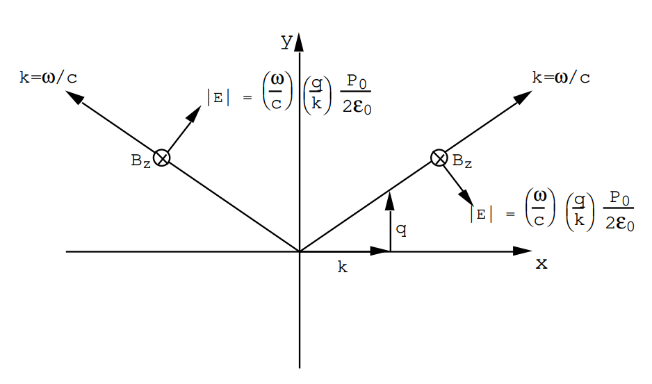
\[\text{B}_{\text{z}}=-\frac{\partial \text{A}_{\text{X}}}{\partial \text{y}}=-\frac{\text{i} \omega \mu_{0} \text{P}_{0}}{2}\left(\frac{\text{q}}{\text{k}}\right) \text{e}^{\text{i}(\text{kx}+\text{qy}-\omega \text{t})}.\nonumber\]

The amplitude of the electric field is

\[|\text{E}|=\sqrt{\text{E}_{\text{x}}^{2}+\text{E}_{\text{Y}}^{2}}=\left(\frac{\omega}{\text{c}}\right)\left(\frac{\text{q}}{\text{k}}\right) \frac{\text{P}_{0}}{2 \varepsilon_{0}},\nonumber\]

therefore cB_z= |E| which is the correct ratio for a plane wave propagating through empty space. A similar calculation shows that a plane wave propagates to the left; its B field is the same as the wave propagating to the right. See the diagram below.

Problem (8.10).

The electron on a hydrogen atom is characterized by the resonant frequency f_o = 15 x 10¹⁵ Hz. The dipole moment induced on each hydrogen atom by an electric field can be written p = \(\alpha\)E where \(\alpha\) is the polarizability.

(a) Estimate the polarizability of a hydrogen atom for an electric field oscillating at a frequency of 10¹⁸ Hz.

(b) Consider a hydrogen atom at the origin. A plane wave is incident on the atom where E_z = E_o e ^i(kx-wt) where E_o = 1 Volt/meter and ω = 2\(\pi\) x 10¹⁸ rad/sec. How large are the electric field components measured by an observer 1 meter distant and located in the x-y plane?

Answer (8.10).

(a) The equation of motion of the electron on the H atom can be written

\[m \frac{d^{2} z}{d t^{2}}+k z=|e| E_{0} e^{-i w t}\nonumber\]

or

\[\frac{d^{2} z}{d t^{2}}+\frac{k}{m} z=-\frac{|e|}{m} E_{0} e^{-i \omega t}.\nonumber\]

The resonant frequency is \(\frac{3}{2} \times 10^{16} \text{Hz}\) therefore \(\frac{\text{k}}{\text{m}}=\left(3 \pi \times 10^{16}\right)^{2}(\text{rad} / \text{sec})^{2}=\Omega^{2}\).

If \(z=z_{0} e^{-i \omega t}\) then \(z_{0}=\frac{-(|e| / m) E_{0}}{\left(\Omega^{2}-\omega^{2}\right)}\).

The dipole moment is \(P_{z}=-|e| z=\frac{\left(e^{2} / m\right)}{\left(\Omega^{2}-\omega^{2}\right)} E_{0} e^{-i \omega t}\),

\(\therefore \alpha=\frac{e^{2} / m}{\left(\Omega^{2}-\omega^{2}\right)} \simeq-\frac{e^{2}}{m \omega^{2}}\) since ω² >> Ω² .

At f = 10¹⁸ Hz ω = 6.28 x 10¹⁸ and \(\alpha\) = - 0.714 x 10^-45 Coulomb meters.

The induced dipole moment is P_z = \(\alpha\)E_z. For an observer in the x-y plane

\[\begin{array}{lll}\theta=\frac{\pi}{2} & \therefore \quad \cos \theta=0 \\& \quad \quad \sin \theta=1\end{array}\nonumber\]

There is no radial component of electric field!

\[E_{\theta}=\frac{1}{4 \pi \varepsilon_{0}}\left[\frac{P_{z}}{R^{3}}+\frac{\dot{P}_{z}}{c R^{2}}+\frac{\ddot{P}_{z}}{c^{2} R}\right]\nonumber\]

Now \(\frac{\omega}{c}=2.09 \times 10^{10}\) \(\left(\frac{\omega}{c}\right)^{2}=4.39 \times 10^{20}\)

So the quantities 1 & \( \frac{\omega}{\mathrm{c}}\) are negligible c.f. \(\left(\frac{\omega}{c}\right)^{2}\)

\(\text{E}_{\theta}=-\frac{(0.71)\left(10^{-45}\right)(1)}{4 \pi \varepsilon_{0}}\left(4.39 \times 10^{20}\right)=\mathbf{-2.82 \times 10^{-15}}\) Volts/meter.

Problem (8.11).

A short thin-wire center-fed dipole antenna of length L meters is oriented along the z-axis with its center at the origin as shown in the sketch.

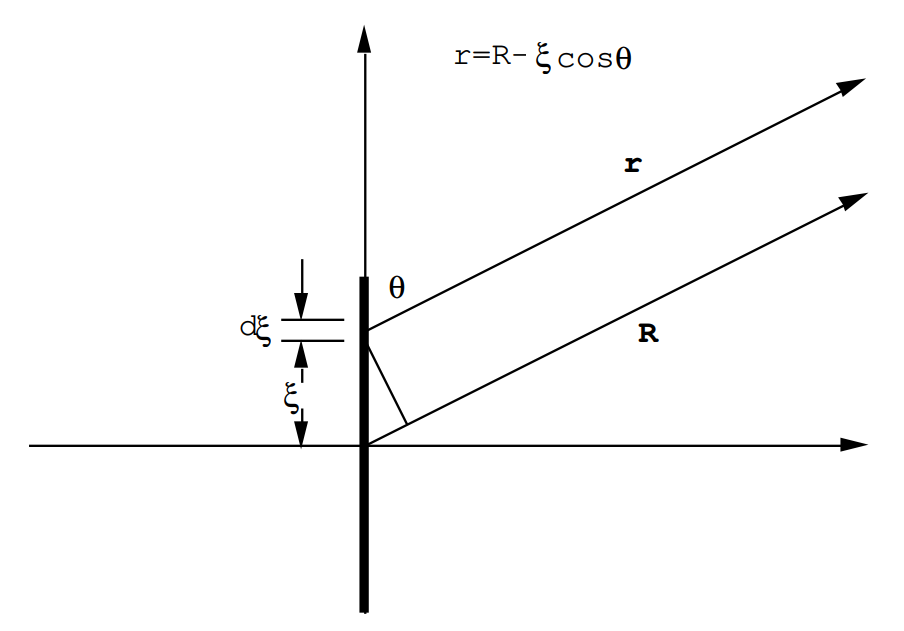
The current distribution on the antenna is given by:

\[z>0: \quad \quad I(\xi)=I_{0}\left(1-\frac{2 \xi}{L}\right) e^{-i \omega t}\nonumber\]

\[z<0: \quad \quad I(\xi)=I_{0}\left(1+\frac{2 \xi}{L}\right) e^{-i \omega t}.\nonumber\]

Show that the radiation resistance of the antenna is given by

\[\text{R}=20 \pi^{2}\left(\frac{\text{L}}{\lambda}\right)^{2} \text { Ohms }.\nonumber\]

Hint: The distance from the element dξ to the observer is given approximately by

\[r=R-\xi \cos \theta=R\left(1-\frac{\xi \cos \theta}{R}\right); \nonumber\]

here ξ/R is a very small quantity. Expand all relevant terms as a power series in (ξ/R) and keep only terms proportional to (ξ/R). Also use the approximation that \(e^{-i \omega \xi \cos \theta / c}\) can be set equal to \(\left(1-i \frac{\omega \xi}{c} \cos \theta\right)\).

Answer (8.11).

\[\text{d} \text{A}_{\text{z}}=\frac{\mu_{0}}{4 \pi} \frac{\text{d} \xi \text{I}(\xi)}{(\text{R}-\xi \cos \theta)} \text{e}^{-\text{i} \omega\left(\text{t}-\frac{\text{R}}{\text{c}}+\frac{\xi \cos \theta}{\text{c}}\right)},\nonumber\]

\[\mathrm{A}_{\mathrm{z}} \cong\left\{\frac{\mu_{0}}{4 \pi \mathrm{R}} \int_{-\mathrm{L} / 2}^{\mathrm{L} / 2} \mathrm{d} \xi \left(1+\frac{\xi_{\mathrm{cos}} \theta}{\mathrm{R}}\right) \mathrm{I}(\xi) e^{\frac{-\mathrm{i} \omega \xi}{\mathrm{c}}} \cos \theta_{\}} \mathrm{e}^{-\mathrm{i} \omega(\mathrm{t}-\mathrm{R} / \mathrm{c})}\right. . \nonumber\]

Drop the term \(e^{-i \omega(t-R / c)}\); it is just a factor throughout.

Let \(e^{-i \omega \xi \cos \theta / c}=(1-i \omega \xi \cos \theta / c)\). Then setting k=ω/c, one finds

\[\text{A}_{\text{z}} \cong \frac{\mu_{0} \text{I}_{0}}{4 \pi \text{R}} \quad \int_{0}^{\text{L/2}} \text{d} \xi \quad\left(1-\frac{2 \xi}{\text{L}}\right)\left(1+\frac{\xi \cos \theta}{\text{R}}\right)(1-\text{i} \text{k} \xi \cos \theta)+\frac{\mu_{0} I_{0}}{4 \pi \text{R}} \int_{-\text{L} / 2} d \xi\left(1+\frac{2 \xi}{\text{L}}\right)\left(1+\frac{\xi \cos \theta}{\text{R}}\right)(1-i \text{k} \xi \cos \theta)\nonumber\]

where \(\frac{\xi}{\text{R}}<<1\) and it is assumed that kξ<<1. With these approximations

\[\text{A}_{\text{z}}=\frac{\mu_{0} \text{I}_{0}}{4 \pi \text{R}} \left(\frac{\text{L}}{2}\right) \text{e}^{-\text{i} \omega[\text{t}-\text{R} / \text{c}]}.\nonumber\]

In spherical polar co-ordinates

\[\begin{equation}\text{A}_{\text{R}}=\frac{\mu_{0} \text{I}_{0}}{4 \pi}\left(\frac{\text{L}}{2}\right) \frac{\cos \theta}{\text{R}} e^{-\text{i} \omega[\text{t}-\text{R} / \text{c}]}\end{equation},\nonumber\]

\[\begin{equation}\text{A}_{\theta}=-\frac{\mu_{0} \text{I}_{0}}{4 \pi}\left(\frac{\text{L}}{2}\right) \frac{\sin \theta}{\text{R}} e^{-\text{i} \omega[\text{t}-\text{R} / \text{c}]}\end{equation}.\nonumber\]

B= curlA. In this case B has only the component B_\(\phi\). The radiation component of this field is proportional to 1/R and is

\[ B_{\phi}=-i \frac{\mu_{0} I_{0}}{4 \pi}\left(\frac{L}{2}\right)\left(\frac{\omega}{c}\right) \frac{\sin \theta}{R} e^{-i \omega[t-R / c]}.\nonumber\]

The electric field is

\(\mathrm{E}_{\theta}=\mathrm{cB}_{\phi}=-\mathrm{i} \frac{\mu_{0} \mathrm{I}_{0}}{4 \pi}\left(\frac{\mathrm{L}}{2}\right) (\omega) \frac{\sin \theta}{\mathrm{R}} e^{-\mathrm{i} \omega[\mathrm{t}-\mathrm{R} / \mathrm{c}]}\).

\(H_{\phi}=B_{\phi} / \mu_{0}=-i \frac{I_{0}}{4 \pi}\left(\frac{L}{2}\right) \left(\frac{\omega}{c}\right) \frac{\sin \theta}{R} e^{-i \omega[t-R / c]}\).

The time average of the Poynting vector, <S_R> is

\( \begin{equation}\left\langle S_{R}\right\rangle=\frac{1}{2} \operatorname{Real}\left(E_{\theta} H_{\phi}^{*}\right)=\frac{1}{2} \frac{\mu_{0} I_{0}^{2}}{16 \pi^{2}} \frac{L^{2}}{4} \frac{\omega^{2}}{c} \frac{\sin ^{2} \theta}{R^{2}}\end{equation}\).

Integrate this expression over the sphere of radius R to get the total radiated power:

\[\begin{equation}\langle\text{P}\rangle=\left(\frac{\pi}{12}\right)\left(\text{CH}_{0}\right)\left(\frac{\text{I}_{0}^{2} \text{L}^{2}}{\lambda^{2}}\right) \text { Watts }\end{equation} \nonumber.\]

But cµ₀= 120\(\pi\), and by definition the radiation resistance R_R is such that \(\begin{equation}\langle P\rangle=\frac{I_{0}^{2} R_{R}}{2}\end{equation} \), therefore

\[ \begin{equation}\text{R}_{\text{R}}=20 \pi^{2}\left(\frac{\text{L}}{\lambda}\right)^{2} \text { Ohms }\end{equation}\nonumber.\]