10.12: Equivalent Circuit Model for Reception, Redux

Section 10.9 provides an informal derivation of an equivalent circuit model for a receiving antenna. This model is shown in Figure \(\PageIndex{1}\).

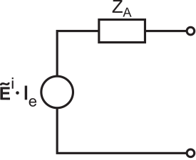Figure \(\PageIndex{1}\): Thévenin equivalent circuit model for an antenna in the presence of an incident electric field \(\mathbf{E}^{i}\). (CC BY-SA 4.0; S. Lally)

The derivation of this model was informal and incomplete because the open-circuit potential \({\bf E}^i\cdot{\bf l}_e\) and source impedance \(Z_A\) were not rigorously derived in that section. While the open-circuit potential was derived in Section 10.11 (“Potential Induced in a Dipole”), the source impedance has not yet been addressed. In this section, the source impedance is derived, which completes the formal derivation of the model. Before reading this section, a review of Section 10.10 (“Reciprocity”) is recommended.

The starting point for a formal derivation is the two-port model shown in Figure \(\PageIndex{2}\).

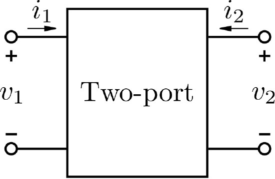Figure \(\PageIndex{2}\): Two-port system. (public domain (modified); Inductiveload)

If the two-port is passive, linear, and time-invariant, then the potential \(v_2\) is a linear function of potentials and currents present at ports 1 and 2. Furthermore, \(v_1\) must be proportional to \(i_1\), and similarly \(v_2\) must be proportional to \(i_2\), so any pair of “inputs” consisting of either potentials or currents completely determines the two remaining potentials or currents. Thus, we may write:

\[v_2 = Z_{21} i_1 + Z_{22} i_2 \label{m0216_ev2} \]

where \(Z_{11}\) and \(Z_{12}\) are, for the moment, simply constants of proportionality. However, note that \(Z_{11}\) and \(Z_{12}\) have SI base units of \(\Omega\), and so we refer to these quantities as impedances. Similarly we may write:

\[v_1 = Z_{11} i_1 + Z_{12} i_2 \label{m0216_ev1} \]

We can develop expressions for \(Z_{12}\) and \(Z_{21}\) as follows. First, note that \(v_{1}=Z_{12}i_2\) when \(i_1=0\). Therefore, we may define \(Z_{12}\) as follows:

\[Z_{12} \triangleq \left.\frac{v_1}{i_2}\right|_{i_1=0} \nonumber \]

The simplest way to make \(i_1=0\) (leaving \(i_2\) as the sole “input”) is to leave port 1 open-circuited. In previous sections, we invoked special notation for these circumstances. In particular, we defined \(\widetilde{I}_2^t\) as \(i_2\) in phasor representation, with the superscript “\(t\)” (“transmitter”) indicating that this is the sole “input”; and \(\widetilde{V}_1^r\) as \(v_1\) in phasor representation, with the superscript “\(r\)” (“receiver”) signaling that port 1 is both open-circuited and the “output.” Applying this notation, we note:

\[Z_{12} = \frac{\widetilde{V}_1^r}{\widetilde{I}_2^t} \label{m0216_eZ12} \]

Similarly:

\[Z_{21} = \frac{\widetilde{V}_2^r}{\widetilde{I}_1^t} \label{m0216_eZ21} \]

In Section 10.10 (“Reciprocity”), we established that a pair of antennas could be represented as a passive linear time-invariant two-port, with \(v_1\) and \(i_1\) representing the potential and current at the terminals of one antenna (“antenna 1”), and \(v_2\) and \(i_2\) representing the potential and current at the terminals of another antenna (“antenna 2”). Therefore for any pair of antennas, quantities \(Z_{11}\), \(Z_{12}\), \(Z_{22}\), and \(Z_{21}\) can be identified that completely determine the relationship between the port potentials and currents.

We also established in Section 10.10 that:

\[\widetilde{I}_1^t \widetilde{V}_1^r = \widetilde{I}_2^t \widetilde{V}_2^r \label{m0216_eRIV} \]

Therefore,

\[\frac{\widetilde{V}_1^r}{\widetilde{I}_2^t} = \frac{\widetilde{V}_2^r}{\widetilde{I}_1^t} \label{m0216_eR1} \]

Referring to Equations \ref{m0216_eZ12} and \ref{m0216_eZ21}, we see that Equation \ref{m0216_eR1} requires that:

\[Z_{12} = Z_{21} \nonumber \]

This is a key point. Even though we derived this equality by open-circuiting ports one at a time, the equality must hold generally since Equations \ref{m0216_ev2} and \ref{m0216_ev1} must apply – with the same values of \(Z_{12}\) and \(Z_{21}\) – regardless of the particular values of the port potentials and currents.

We are now ready to determine the Thévenin equivalent circuit for a receiving antenna. Let port 1 correspond to the transmitting antenna; that is, \(i_1\) is \(\widetilde{I}_1^t\). Let port 2 correspond to an open-circuited receiving antenna; thus, \(i_2=0\) and \(v_2\) is \(\widetilde{V}_2^r\). Now applying Equation \ref{m0216_ev2}:

\[\begin{aligned} v_2 &= Z_{21} i_1 + Z_{22} i_2 \nonumber \\ &= \left(\widetilde{V}_2^r/\widetilde{I}_1^t\right) \widetilde{I}_1^t + Z_{22} \cdot 0 \nonumber \\ &= \widetilde{V}_2^r\end{aligned} \nonumber \]

We previously determined \(\widetilde{V}_2^r\) from electromagnetic considerations to be (Section 10.11):

\[\widetilde{V}_2^r = \widetilde{\bf E}^i\cdot{\bf l}_e \nonumber \]

where \(\widetilde{\bf E}^i\) is the field incident on the receiving antenna, and \({\bf l}_e\) is the vector effective length as defined in Section 10.11. Thus, the voltage source in the Thévenin equivalent circuit for the receive antenna is simply \(\widetilde{\bf E}^i\cdot{\bf l}_e\), as shown in Figure \(\PageIndex{1}\).

The other component in the Thévenin equivalent circuit is the series impedance. From basic circuit theory, this impedance is the ratio of \(v_2\) when port 2 is open-circuited (i.e., \(\widetilde{V}_2^r\)) to \(i_2\) when port 2 is short-circuited. This value of \(i_2\) can be obtained using Equation \ref{m0216_ev2} with \(v_2=0\):

\[0 = Z_{21} \widetilde{I}_1^t + Z_{22} i_2 \nonumber \]

Therefore:

\[i_2 = - \frac{Z_{21}}{Z_{22}} \widetilde{I}_1^t \nonumber \]

Now using Equation \ref{m0216_eZ21} to eliminate \(\widetilde{I}_1^t\), we obtain:

\[i_2 = - \frac{\widetilde{V}_2^r}{Z_{22}} \nonumber \]

Note that the reference direction for \(i_2\) as defined in Figure \(\PageIndex{2}\) is opposite the reference direction for short-circuit current. That is, given the polarity of \(v_2\) shown in Figure \(\PageIndex{2}\), the reference direction of current flow through a passive load attached to this port is from “\(+\)” to “\(-\)” through the load. Therefore, the source impedance, calculated as the ratio of the open-circuit potential to the short circuit current, is:

\[\frac{\widetilde{V}_2^r}{+\widetilde{V}_2^r/Z_{22}} = Z_{22} \nonumber \]

We have found that the series impedance \(Z_A\) in the Thévenin equivalent circuit is equal to \(Z_{22}\) in the two-port model.

To determine \(Z_{22}\), let us apply a current \(i_2=\widetilde{I}_2^t\) to port 2 (i.e., antenna 2). Equation \ref{m0216_ev2} indicates that we should see:

\[v_2 = Z_{21} i_1 + Z_{22} \widetilde{I}_2^t \nonumber \]

Solving for \(Z_{22}\):

\[Z_{22} = \frac{v_2}{\widetilde{I}_2^t} - Z_{21} \frac{i_1}{\widetilde{I}_2^t} \label{m0216_eZ22exact} \]

Note that the first term on the right is precisely the impedance of antenna 2 in transmission. The second term in Equation \ref{m0216_eZ22exact} describes a contribution to \(Z_{22}\) from antenna 1. However, our immediate interest is in the equivalent circuit for reception of an electric field \(\widetilde{\bf E}^i\) in the absence of any other antenna. We can have it both ways by imagining that \(\widetilde{\bf E}^i\) is generated by antenna 1, but also that antenna 1 is far enough away to make \(Z_{21}\) – the factor that determines the effect of antenna 1 on antenna 2 – negligible. Then we see from Equation \ref{m0216_eZ22exact} that \(Z_{22}\) is the impedance of antenna 2 when transmitting.

Summarizing:

The Thévenin equivalent circuit for an antenna in the presence of an incident electric field \(\widetilde{\bf E}^i\) is shown in Figure \(\PageIndex{1}\). The series impedance \(Z_A\) in this model is equal to the impedance of the antenna in transmission.

Mutual coupling

This concludes the derivation, but raises a follow-up question: What if antenna 2 is present and not sufficiently far away that \(Z_{21}\) can be assumed to be negligible? In this case, we refer to antenna 1 and antenna 2 as being “coupled,” and refer to the effect of the presence of antenna 1 on antenna 2 as coupling. Often, this issue is referred to as mutual coupling, since the coupling affects both antennas in a reciprocal fashion. It is rare for coupling to be significant between antennas on opposite ends of a radio link. This is apparent from common experience. For example, changes to a receive antenna are not normally seen to affect the electric field incident at other locations. However, coupling becomes important when the antenna system is a dense array; i.e., multiple antennas separated by distances less than a few wavelengths. It is common for coupling among the antennas in a dense array to be significant. Such arrays can be analyzed using a generalized version of the theory presented in this section.