1.4: Ampere’s Law and Magnetostatic Fields

The relevant Maxwell’s equation for static current densities \(\vec J\) [A/m² ] is Ampere’s law, which says that for time-invariant cases the integral of magnetic field \(\vec H\) around any closed contour in a right-hand sense equals the area integral of current density \(\vec J\) [A/m² ] flowing through that contour:

\[\oint_{\mathrm{c}} \vec{\mathrm{H}} \cdot \mathrm{d} \vec{\mathrm{s}}=\int \int_{\mathrm{A}} \vec{\mathrm{J}} \cdot \mathrm{d} \vec{\mathrm{a}}\]

Figure 1.4.1 illustrates a simple cylindrical geometry for which we can readily compute \(\vec H\) produced by current I; the radius of the cylinder is R and the uniform current density flowing through it is J_o [A/m² ]. The cylinder is infinitely long.

Figure 1.4.1: Magnetic field produced by a uniform cylindrical current.

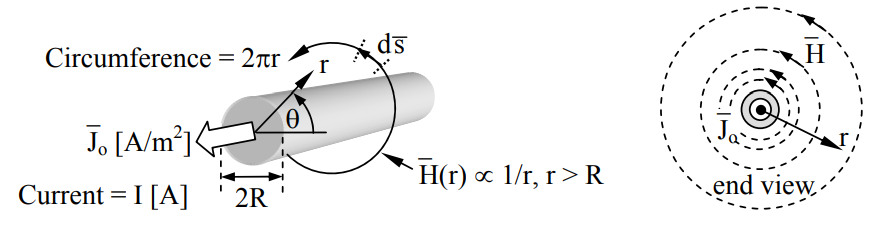
Because the problem is cylindrically symmetric (not a function of θ), and uniform with respect to the cylindrical axis z, so is the solution. Thus \(\vec H\) depends only upon radius r. Substitution of \(\vec H\)(r) into (1.4.1) yields:

\[\int_{0}^{2 \pi} \vec{\mathrm{H}}(\mathrm{r}) \cdot \hat{\theta} \mathrm{rd} \theta=\int_{0}^{2 \pi} \int_{0}^{\mathrm{R}} \mathrm{J}_{\mathrm{o}} \mathrm{r} \mathrm{dr} \mathrm{d} \theta=\mathrm{J}_{\mathrm{o}} \pi \mathrm{R}^{2}=\mathrm{I}[\mathrm{A}]\]

where the total current I is simply the uniform current density J_o times the area πR² of the cylinder. The left-hand-side of (1.4.2) simply equals H(r) times the circumference of a circle of radius r, so (1.4.2) becomes:

\[\int_{0}^{2 \pi} \vec{\mathrm{H}}(\mathrm{r}) \cdot \hat{\theta} \mathrm{rd} \theta=\int_{0}^{2 \pi} \int_{0}^{\mathrm{R}} \mathrm{J}_{\mathrm{O}} \mathrm{r} \mathrm{dr} \mathrm{d} \theta=\mathrm{J}_{\mathrm{o}} \pi \mathrm{R}^{2}=\mathrm{I}[\mathrm{A}]\]

Within the cylindrical wire where r < R, (1.4.2) becomes:

\[\vec{\mathrm{H}}(\mathrm{r})=\hat{\theta} \frac{\mathrm{I}}{2 \pi \mathrm{r}}=\hat{\theta} \frac{\mathrm{J}_{0} \pi \mathrm{R}^{2}}{2 \pi \mathrm{r}}[\mathrm{A} / \mathrm{m}] \quad \quad \quad (\mathrm{r}>\mathrm{R}) \]

\[\vec{\mathrm{H}}(\mathrm{r})=\hat{\theta} \mathrm{J}_{\mathrm{o}} \mathrm{r} / 2[\mathrm{A} / \mathrm{m}] \quad \quad \quad(\mathrm{r}<\mathrm{R})\]

Therefore H(r) increases linearly with r within the wire and current distribution, and is continuous at r = R, where both (1.4.3) and (1.4.5) agree that H(r) = J_oR/2.

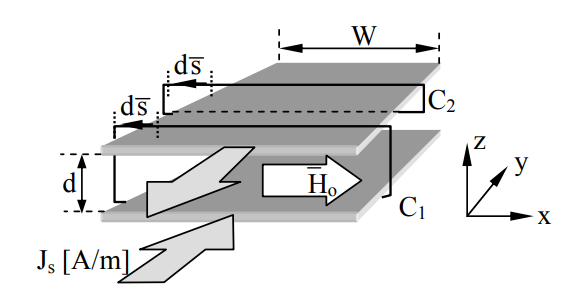
Another simple geometry involves parallel plates. Assume equal and opposite current densities, J_s [A/m], flow in infinite parallel plates separated by distance d, as illustrated in Figure 1.4.2 for finite plates. The integral of Ampere’s law (1.4.1) around any contour C₁ circling both plates is zero because the net current through that contour is zero. A non-zero integral would require an external source of field, which we assume does not exist here. Thus \(\vec H\) above and below the plates is zero. Since the integral of (1.4.1) around any contour C₂ that circles the upper plate yields HxW = J_sW, where the x component of the magnetic field anywhere between the plates is H_x = J_s [A/m]; thus the magnetic field \(\vec H\) between the plates is uniform. An integral around any contour in any y-z plane would circle no net current, so H_z = 0, and a similar argument applies to H_y, which is also zero. This configuration is discussed further in Section 3.2.1.

Figure 1.4.2: Static magnetic field between parallel plates.

More generally, because Maxwell’s equations are linear, the total magnetic field \(\vec H\) at any location is the integral of contributions made by current densities \(\vec J\) nearby. Section 10.1 proves the Biot-Savart law (1.4.6), which defines how a current distribution \(\vec J\)' at position \(\vec r\)' within volume V' contributes to \(\vec H\) at position \(\vec r\):

\[\vec{\mathrm{H}}(\vec{\mathrm{r}}, \mathrm{t})=\int \int \int_{\mathrm{V}^{\prime}} \frac{\vec{\mathrm{J}}^{\prime} \times\left(\vec{\mathrm{r}}-\overrightarrow{\mathrm{r}}^{\prime}\right)}{4 \pi\left|\vec{\mathrm{r}}-\overrightarrow{\mathrm{r}}^{\prime}\right|^{3}} \mathrm{d} \mathrm{v}^{\prime} \quad \quad \quad \quad \quad (Biot-Savart \quad law) \]

To summarize, electric and magnetic fields are simple fictions that explain all electromagnetic behavior as characterized by Maxwell’s equations and the Lorentz force law, which are examined further in Chapter 2. A simple physical model for the static behavior of electric fields is that of rubber bands that tend to pull opposite electric charges toward one another, but that tend to repel neighboring field lines laterally. Static magnetic fields behave similarly, except that the role of magnetic charges (which have not been shown to exist) is replaced by current loops acting as magnetic dipoles in ways that are discussed later.