4.4: A Second Approach to Magnetostatics

When time variations of the source terms can be neglected we have seen that Maxwell’s equations for the magnetostatic field become

\[\operatorname{div}(\overrightarrow{\mathrm{B}})=0 \label{4.31}\]

\[\operatorname{curl}(\overrightarrow{\mathrm{B}})=\mu_{0}\left(\overrightarrow{\mathrm{J}}_{f}+\operatorname{curl}(\overrightarrow{\mathrm{M}})\right). \label{4.32}\]

The auxillary vector \(\vec H\) was introduced in chapter(1), section(1.4), through the relation

\[\overrightarrow{\mathrm{B}}=\mu_{0}(\overrightarrow{\mathrm{H}}+\overrightarrow{\mathrm{M}}). \label{4.33}\]

When (\ref{4.33}) is used in (\ref{4.31}) and (\ref{4.32}) to replace \(\vec B\) by \(\vec H\) the result is

\[\operatorname{curl}(\overrightarrow{\mathrm{H}})=\overrightarrow{\mathrm{J}}_{f} \label{4.34}\]

\[\operatorname{div}(\overrightarrow{\mathrm{H}})=-\operatorname{div}(\overrightarrow{\mathrm{M}}). \label{4.35}\]

For problems in which there is no free current density, \(\vec J\)_f , these equations reduce to

\[\operatorname{curl}(\overrightarrow{\mathrm{H}})=0, \label{4.36}\]

\[\operatorname{div}(\overrightarrow{\mathrm{H}})=-\operatorname{div}(\overrightarrow{\mathrm{M}})=\rho_{\mathrm{M}}. \label{4.37}\]

The form of these equations for the field \(\vec H\) is exactly the same as the form of Maxwell’s equations for the electrostatic field in the absence of a free charge density, ie. (see section(2.1))

\[\operatorname{curl}(\overrightarrow{\mathrm{E}})=0, \nonumber \]

\[\operatorname{div}(\overrightarrow{\mathrm{E}})=-\frac{1}{\epsilon_{0}} \operatorname{div}(\overrightarrow{\mathrm{P}})=\frac{\rho_{b}}{\epsilon_{0}}. \nonumber\]

The analogy between these equations for the electrostatic field and the above equations for the magnetic field, \(\vec H\), in a current free region suggests that \(\vec H\) can be obtained from a magnetic potential function, \(\mathrm{V}_{\mathrm{M}} ; \overrightarrow{\mathrm{H}}=-\operatorname{grad}\left(\mathrm{V}_{\mathrm{M}}\right)\). Notice that if there are no free currents, curlH=0, and therefore in the absence of a current density the tangential components of H must be continuous everywhere. The truth of this statement can be demonstrated by means of an application of Stokes’ theorem, section(1.3.4). The argument is the same as that used to derive Equation (2.4.1) which states that the tangential component of the electrostatic field must be continuous across a boundary. In the electrostatic case continuity of the tangential component of E can be guaranteed by the requirement that the electrostatic potential function be continuous. In the equivalent magnetostatic case the continuity of the tangential component of H is guaranteed by the requirement that the magnetostatic potential function, V_M, be continuous across a boundary.

The machinery that was set up in Chapter(2) to calculate the electrostatic field from a given charge distribution can be taken over intact to calculate the magnetostatic field from a given ”magnetic charge density” distribution, ρ_M, where

\[\rho_{M}=-\operatorname{div}(\overrightarrow{\mathrm{M}}). \label{4.38}\]

From now on Equation (\ref{4.38}) will be used to define what is meant by the term magnetic charge density. There is no real magnetic charge density; to this date (2004) no one has been able to discover a magnetic monopole, the magnetic analogue of an electric charge. If a magnetic monopole were to be discovered it would have the units of Amp-meters, and it would produce a field

\[\overrightarrow{\mathrm{H}}=\frac{1}{4 \pi} \frac{\mathrm{q}_{\mathrm{m}}}{\mathrm{r}^{2}}\left(\frac{\overrightarrow{\mathrm{r}}}{\mathrm{r}}\right) \quad \text { Amps / meter }, \nonumber\]

by analogy with the electrostatic case, where q_m is the strength of the magnetic charge.

If curl(\(\vec H\)) = 0, ie. no free current density, the magnetic field can be written as the gradient of a magnetic scalar potential, V_M:

\[\overrightarrow{\mathrm{H}}=-\operatorname{grad}\left(\mathrm{V}_{\mathrm{M}}\right). \label{4.39}\]

Eqn.(\ref{4.39}) guarantees that curl(\(\vec H\)) = 0 since the curl of a gradient is always zero. Notice that an arbitrary constant can be added to the potential without changing the magnetic field, \(\vec H\). This constant is usually chosen to make the expression for the potential function as simple as possible. Upon substituting Equation (\ref{4.39}) into Equation (\ref{4.37}) for the divergence of \(\vec H\) one obtains

\[\operatorname{div} \operatorname{grad}\left(\mathrm{V}_{\mathrm{M}}\right)=-\rho_{\mathrm{M}} , \nonumber \]

or

\[\nabla^{2} \mathrm{V}_{\mathrm{M}}=-\rho_{M} . \label{4.40}\]

By analogy with the electrostatic case, Equation (2.2.4), the particular solution for the magnetic potential can be written

\[\mathrm{V}_{\mathrm{M}}(\overrightarrow{\mathrm{R}})=\frac{1}{4 \pi} \iiint_{S p a \infty} \mathrm{d} \mathrm{Vol} \frac{\rho_{M}(\overrightarrow{\mathrm{r}})}{|\overrightarrow{\mathrm{R}}-\overrightarrow{\mathrm{r}}|}. \label{4.41}\]

In the application of Equation (\ref{4.41}) it must be remembered that a discontinuity in the normal component of the magnetization, \(\vec M\), will produce a surface density of magnetic charges just as a discontinuity in the normal component of the electric dipole moment, \(\vec P\), produces a surface density of bound electric charges, Chapter(2), section(2.3.3). The magnetic surface charge density contributes to the magnetic potential, V_M(\(vec R\)), and must be included in Equation (\ref{4.41}) as a surface integral. It is often easier to calculate the fields generated by a given configuration of magnetization density by means of the magnetic scalar potential than it is to use the equivalent current density, \(\vec J\)_f = curl(\(\vec M\)), and the generalized law of Biot-Savart, Equation (4.1.15). Examples follow of magnetic field distributions calculated from given magnetization distributions using the magnetic scalar potential.

4.4.1 An Infinitely Long Uniformly Magnetized Rod.

See Figure (4.3.11). For this case div(\(\vec M\)) = 0 everywhere, so that ρ_M = 0 everywhere. There are no surface charge densities because there are no discontinuities in the normal component of \(\vec M\). This means that the magnetic potential must be independent of position, see Equation (\ref{4.41}), and thus

\[\overrightarrow{\mathrm{H}}=-\operatorname{grad}\left(\mathrm{V}_{\mathrm{M} 1}\right)=0. \nonumber \]

But by definition

\[\overrightarrow{\mathrm{H}}=\left(\frac{\overrightarrow{\mathrm{B}}}{\mu_{0}}-\overrightarrow{\mathrm{M}}\right) , \nonumber \]

therefore if \(\vec H\) = 0 it follows that \(\vec B\) = µ₀\(\vec M\) in agreement with Equation (4.3.11) which was earlier obtained using the law of Biot and Savart;(see section(4.3.7) above).

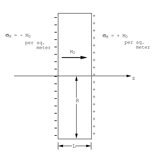
4.4.2 A Thin Disc Uniformly Magnetized along its Axis.

Consider a disc of radius R meters and having a thickness of L meters, that is uniformly magnetized parallel with its axis as shown in Figure (4.4.12); M_z = M₀. The discontinuity in the normal component of the magnetization at the front and rear surfaces produces a surface magnetic charge density given by σ_M = +M₀ per m₂ on the front surface and σ_M = −M₀ per m₂ on the rear surface. These magnetic charge densities produce a magnetic field along the axis of the disc that can be obtained from the scalar potential, V_M, calculated using Equation (\ref{4.41}), where, for this example, the volume integral reduces to a surface integral. The field \(\vec H\) so calculated can be used to calculate \(\vec B\) along the axis: the result is given by Equation (4.3.12) of section(4.3.8).

If (R/L) ≫ 1 the configuration of charges illustrated in Figure (4.4.12) is the magnetic analogue of the electrostatic double layer problem, section(2.7.1) example(4), Figures (2.7.9) and (2.7.10). By analogy with the electrostatic double layer, one can immediately deduce that outside the disc the magnetic field \(\vec H\) is zero, but inside the disc H_z = −M₀. From the definition \(\overrightarrow{\mathrm{B}}=\mu_{0}(\overrightarrow{\mathrm{H}}+\overrightarrow{\mathrm{M}})\) this means that, for a disc having an infinite radius, the field \(\vec B\) is zero both inside and outside the disc. This conclusion is in agreement with Equation (4.3.12) in which the field \(\vec B\) was calculated along the axis from the equivalent surface current density on the edge of the disc. Notice that the normal component of \(\vec B\) is continuous across the interface between the outside and inside of the magnet. It is a general consequence of the Maxwell equation div(\(\vec B\)) = 0 that the normal component of B must be continuous across any interface.

Figure \(\PageIndex{12}\): A uniformly magnetized disc. The discontinuities in the normal component of the magnetization generate an effective magnetic surface charge density on the front and back surfaces of the disc.

4.4.3 A Uniformly Magnetized Ellipsoid.

The results of section(2.7.4) for a uniformly polarized ellipsoid can be taken over for the magnetic case because of the similarity between the equations for the electrostatic field, \(\vec E\), and those for the magnetic field, \(\vec H\), in a current free region. Consider the ellipsoid whose surface is described by

\[\left(\frac{x}{a}\right)^{2}+\left(\frac{y}{b}\right)^{2}+\left(\frac{z}{c}\right)^{2}=1. \nonumber \]

Let the components of the magnetization in the principle axis system be M_x, M_y, M_z. There exist demagnetizing coefficients, N_\(\alpha\), such that the field \(\vec H\) inside the ellipsoid is uniform with

\[\begin{array}{l}
\mathrm{H}_{\mathrm{x}}=-\mathrm{N}_{\mathrm{x}} \mathrm{M}_{\mathrm{x}}, \\
\mathrm{H}_{\mathrm{y}}=-\mathrm{N}_{\mathrm{y}} \mathrm{M}_{\mathrm{y}}, \\
\mathrm{H}_{\mathrm{z}}=-\mathrm{N}_{\mathrm{z}} \mathrm{M}_{\mathrm{z}}.
\end{array} \label{4.42}\]

Moreover, the demagnetizing coefficients satisfy the sum rule

\[\mathrm{N}_{\mathrm{x}}+\mathrm{N}_{\mathrm{y}}+\mathrm{N}_{\mathrm{z}}=1. \label{4.43}\]

Equations (\ref{4.42}) and (\ref{4.43}) are the magnetic analogues of eqns,(2.7.5) and (2.7.6) for a uniformly polarized ellipsoid in the electrostatic case. Demagnetizing factors for simple degenerate limits of the ellipsoid of revolution can be deduced immediately from the sum rule and symmetry arguments, just as for the electrostatic case:

(1) A uniformly magnetized sphere: N_x = N_y = N_z = 1/3.

(2) A long cylinder magnetized transverse to its axis. In this case the demagnetizing factor for the long axis, the z-axis say, is zero, ie. N_z = 0. Therefore since the other two demagnetizing factors are equal, one must have N_x = N_y = 1/2.

(3) A flat disc having a very large radius and magnetized along its axis. In the limit of infinite radius the in-plane demagnetizing factors go to zero, and therefore from the sum rule N_z = 1.

For the general ellipsoid the demagnetizing factors are given by Equations (2.7.11), and for ellipsoids of revolution by Equations (2.7.7 and 2.7.9).

The magnetic field \(\vec H\) outside a uniformly magnetized ellipsoid is generally not uniform even though the field \(\vec H\) inside the ellipsoid is uniform. Analytical expressions for the field H, and therefore also for the field B, are available but they are complicated and are written using generalized elliptic co-ordinate systems. See Electromagnetic Theory by J.A. Stratton, McGraw-Hill, N.Y., 1941, sections 3.25 to 3.27.

4.4.4 A Magnetic Point Dipole.

By analogy with the electrostatic case, the magnetic field around a point magnetic dipole can be obtained from a magnetic potential function of the form

\[\text{V}_{\text{M}}=\frac{1}{4 \pi}\left(\frac{\vec{\text{m}} \cdot \vec{\text{r}}}{\text{r}^{3}}\right). \label{4.44}\]

This potential function gives the magnetic field

\[\vec{\text{H}}(\vec{\text{r}})=\frac{1}{4 \pi}\left(\frac{3[\vec{\text{m}} \cdot \vec{\text{r}}] \vec{\text{r}}}{\text{r}^{5}}-\frac{\vec{\text{m}}}{\text{r}^{3}}\right). \label{4.45}\]

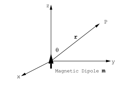
The components of this field when written in the spherical polar co-ordinate system are (see Figure (4.4.13))

\[\text{H}_{\text{r}}=\frac{2 \text{m}}{4 \pi} \frac{\cos \theta}{\text{r}^{3}}, \nonumber \]

\[\text{H}_{\theta}=\frac{\text{m}}{4 \pi} \frac{\sin \theta}{\text{r}^{3}}, \label{4.46}\]

\[\text{H}_{\phi}=0. \nonumber \]

The components of \(\vec B\) are obtained from the components of \(\vec H\) by multiplying by the permeability of free space, µ₀. The resulting expressions are exactly the same as the ones obtained earlier, Equation (4.3.10), from the vector potential for a point dipole, Equation (4.3.9). Thus, the field due to a magnetic point dipole can be calculated either from a magnetic vector potential or from a magnetic scalar potential.

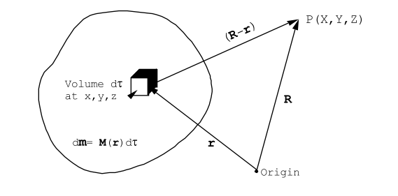
The magnetic scalar potential corresponding to a given distribution of magnetization density can be calculated by superposition using the magnetic

Figure \(\PageIndex{13}\): A magnetic point dipole oriented along the z-axis.

potential due to a point dipole, Equation (\ref{4.44}), see Figure (4.4.14). The element of volume, d\(\tau\), has associated with it a magnetic dipole moment \(\vec{\text{m}}=\vec{\text{M}}(\vec{\text{r}}) \text{d} \tau\). This contributes to the magnetic scalar potential at point P(X,Y,Z) an amount given by

\[\text{dV}_{\text{P}}(\vec{\text{R}})=\frac{1}{4 \pi} \frac{\vec{\text{M}}(\vec{\text{r}}) \cdot[\vec{\text{R}}-\vec{\text{r}}]}{|\vec{\text{R}}-\vec{\text{r}}|^{3}} \text{d} \tau. \label{4.47}\]

Sum Equation (\ref{4.47}) over the entire magnetization distribution to obtain

\[\text{V}_{\text{P}}(\vec{\text{R}})=\frac{1}{4 \pi} \int \int \int_{S p a c e} \text{d} \tau \frac{\vec{\text{M}}(\vec{\text{r}}) \cdot[\vec{\text{R}}-\vec{\text{r}}]}{|\vec{\text{R}}-\vec{\text{r}}|^{3}}. \label{4.48}\]

The potential calculated using Equation (\ref{4.48}) will give the same fields as that calculated from the equivalent magnetic charge distribution and Equation (\ref{4.41}) which is based upon the superposition of the magnetic potentials generated by fictitious point magnetic charges. The proof that the potential calculated in these two different ways is the same, except, possibly for a constant, is based on the identity

\[\operatorname{div}\left(\frac{\pi}{\left(\frac{\pi}{1}-\bar{r}\right)}\right)=\frac{\operatorname{div}(\vec{x})}{|\vec{R}-\vec{r}|}+\vec{11} \cdot \operatorname{grad}\left(\frac{1}{|\vec{R}-\vec{r}|}\right). \nonumber \]

Figure \(\PageIndex{14}\): The calculation of the magnetic scalar potential for a given distribution of magnetization density, \(\vec M\)(\(\vec r\)), using superposition and the potential function for a point magnetic dipole.

The argument proceeds in exactly the same fashion as for the analogous electrostatic case; see Chpt.(2), section(2.8).