
8.3: Power Radiated by a Simple Antenna
- Page ID
- 22841

The radiation fields generated by a simple center-fed linear antenna oriented along the z-axis can be written
\[ \begin{array}{l}
\mathrm{B}_{\phi}=\frac{\mu_{0}}{4 \pi} \mathrm{I}_{0}\left(\frac{\omega}{\mathrm{c}}\right) \cos (\omega[\mathrm{t}-\mathrm{R} / \mathrm{c}]) \frac{\sin \theta \mathrm{F}(\theta)}{\mathrm{R}}, \\
\mathrm{E}_{\theta}=\mathrm{cB}_{\phi}
\end{array}, \label{8.13}\]
where
\[ \sin \theta \mathrm{F}(\theta)=\frac{2}{\left(\frac{\omega}{\mathrm{c}}\right) \sin \theta}\left[\cos \left(\frac{\omega \mathrm{L} \cos \theta}{\mathrm{c}}\right)-\cos \left(\frac{\omega \mathrm{L}}{\mathrm{c}}\right)\right], \label{8.14}\]
(see Chapter(7) Equations (7.3.6 and 7.3.4). The simplest resonant antenna is that for which (ωL/c) = \(\pi\)/2. This is a half-wave antenna for which 2L = λ/2; ie. the total length of the antenna is half the free space wavelength λ = 2\(\pi\)(c/ω) = 2\(\pi\)/k. For this half-wave antenna Equation (7.3.4) becomes
\[\sin \theta \mathrm{F}(\theta)=\frac{2}{\left(\frac{\omega}{c}\right) \sin \theta} \cos \left(\frac{\pi}{2} \cos \theta\right), \label{8.15}\]
and the current distribution along the antenna becomes
\[\mathrm{I}_{\mathrm{z}}(\mathrm{z})=\mathrm{I}_{0} \sin (\omega \mathrm{t}) \cos \left(\frac{\pi \mathrm{z}}{2 \mathrm{L}}\right), \label{8.16}\]
see Figure (8.2.2). The Poynting vector is SR = (EθBφ/µ0), and since \(\vec E\) and \(\vec B\) oscillate in phase the time averaged Poynting vector is given by
\[<\mathrm{S}_{\mathrm{R}}>=\frac{\left|\mathrm{E}_{\theta} \| \mathrm{B}_{\phi}\right|}{2 \mu_{0}}, \nonumber \]
where | Eθ | and | Bφ | are the electric and magnetic field amplitudes. For the particular case of the half-wave antenna one finds using (\ref{8.15})
\[<\mathrm{S}_{\mathrm{R}}>=\frac{1}{8 \pi^{2}} \sqrt{\frac{\mu_{0}}{\epsilon_{0}}} \mathrm{I}_{0}^{2} \frac{\cos ^{2}\left(\frac{\pi \cos \theta}{2}\right)}{\mathrm{R}^{2} \sin ^{2} \theta}. \label{8.17}\]
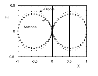
\(\mathrm{Z}_{0}=\sqrt{\mu_{0} / \epsilon_{0}}=120 \pi\) Ohms= 377 Ohms is the impedance of free space. The variation with angle of the radiated power is shown in Figure (8.3.3) where it is compared with the simple sin2 θ pattern characteristic of a point dipole. The total average power passing through a sphere of radius R is independent of R and is given by
\[<\mathrm{P}_{\mathrm{R}}>=2 \pi \mathrm{R}^{2} \int_{0}^{\pi}<\mathrm{S}_{\mathrm{R}}>\sin \theta \mathrm{d} \theta, \nonumber \]
or
\[<\mathrm{P}_{\mathrm{R}}>=30 \mathrm{I}_{0}^{2} \int_{0}^{\pi} \mathrm{d} \theta \frac{\cos ^{2}\left(\frac{\pi}{2} \cos \theta\right)}{\sin \theta}, \nonumber \]
since \(\sqrt{\mu_{0} / \epsilon_{0}}=120 \pi \text { Ohms. }\) The integral can be evaluated numerically. The result is
\[<\mathrm{P}_{\mathrm{R}}>=73.13\left(\frac{\mathrm{I}_{0}^{2}}{2}\right) \quad \text { Watts }. \label{8.18}\]
The average power dissipated in a resistor, R Ohms, by a sinusoidal current having an amplitude I0 Amps is \(\mathrm{R}\left(\mathrm{I}_{0}^{2} / 2\right)\), therefore the ideal halfwave antenna presents an impedance to the power source whose real part is RA= 73.13 Ohms. The resistance RA is called the radiation resistance of the antenna. An ideal antenna is one for which the Ohmic resistance of the antenna wire itself is negligible compared with the radiation resistance. The antenna will also present an inductive or capacitive impedance to the generator since energy is stored in the electric and magnetic near fields. A thin wire half-wavelength antenna has an impedance Z = 73.1+i42.5 Ohms; in other words, the impedance contains an inductive component. However, if the antenna is made 0.49λ long, the impedance becomes purely resistive at approximately 73 Ohms. Such an antenna is said to be tuned. The input impedance of a shorter antenna contains a capacitive component; a longer antenna carries an inductive impedance component. Thus the input impedance of a half-wave dipole antenna varies rapidly with frequency. For practical use it is desirable to construct an antenna that (1) radiates most of its energy into a relatively narrow cone, and (2) one that has an input impedance that is relatively insensitive to frequency. These requirements have led to the development of a large variety of antenna configurations. These are described by John D. Kraus in ”Antennas”, McGraw-Hill, New York, 1988.
An antenna can, of course, also be used to detect the power broadcast by an antenna. It is instructive to examine the problem of an antenna used as a receiver. Let the antenna be terminated by a matched load; the resistive part of the load will thus be equal to the antenna radiation resistance, RA. Let us use the specific example of a half-wave antenna for which RA ≈ 73 Ohms. Assume that the receiving antenna is oriented parallel with the transmitting antenna so that the incident electric field vector is oriented along the receiving antenna: if the \(\vec E\) field is transverse to the antenna no signal will be detected. Usually, the transmitter is so far removed from the receiver that the incident electric field amplitude can be taken as constant over the receiving antenna. Let the amplitude of this incident electric field be E0. The incident electric field will induce a current distribution on the half-wave antenna that has the form described by Equation (\ref{8.16}) and an amplitude IA Amps. Assume that the antenna is connected to a detector whose input impedance has been matched to the antenna impedance. The average rate at which power is extracted from the incident radio wave is
\[<\mathrm{P}_{\mathrm{A}}>=\frac{1}{2} \int_{-\mathrm{L}}^{+\mathrm{L}} \mathrm{d} \mathrm{z} \mathrm{E}_{0} \mathrm{I}_{\mathrm{A}} \cos \left(\frac{\pi \mathrm{z}}{2 \mathrm{L}}\right)=\frac{2 \mathrm{L}}{\pi} \mathrm{E}_{0} \mathrm{I}_{\mathrm{A}} \quad \text { Watts }. \label{8.19}\]
This means that for a half-wave antenna and a matched load the detector resistance will be 73 Ohms. For this matched receiver one half the incident power will be re-radiated (the current distribution will after all radiate away power at the average rate of \(\mathrm{R}_{\mathrm{A}} \mathrm{I}_{\mathrm{A}}^{2} / 2\) Watts), and half the power will be absorbed by the matched detector, \(\mathrm{R}_{\mathrm{A}} \mathrm{I}_{\mathrm{A}}^{2} / 2\) Watts. Thus the useful power picked up by the antenna and delivered to the detector is
\[\mathrm{P}_{\mathrm{D}}=\frac{\mathrm{L}}{\pi} \mathrm{E}_{0} \mathrm{I}_{\mathrm{A}}=\frac{\mathrm{R}_{\mathrm{A}}}{2} \mathrm{I}_{\mathrm{A}}^{2}. \label{8.20}\]
From this equation one finds \(\mathrm{I}_{\mathrm{A}}=2 \mathrm{LE}_{0} /\left(\pi \mathrm{R}_{\mathrm{A}}\right)\), and
\[\mathrm{P}_{\mathrm{D}}=\frac{2 \mathrm{L}^{2}}{\pi^{2}} \frac{\mathrm{E}_{0}^{2}}{\mathrm{R}_{\mathrm{A}}} \quad \text { Watts }. \label{8.21}\]
It is useful and interesting to ask ”how large must a disc be so that all the transmitted energy intercepted by the disc is equal to the power PD delivered to the detector?”. The area of such a disc is called the ”Effective Aperture”, AE, of the receiving antenna. The amplitude of the time-averaged Poynting vector for an incident wave of amplitude E0 is
\[<\mathrm{P}>=\frac{\mathrm{E}_{0}^{2}}{2 \mathrm{c} \mu_{0}}=\frac{\mathrm{E}_{0}^{2}}{2 \mathrm{Z}_{0}} \quad \text { Watts } / \mathrm{m}^{2}, \nonumber \]
where Z0=377 Ohms. Therefore
\[\frac{\mathrm{E}_{0}^{2}}{2 \mathrm{Z}_{0}} \mathrm{A}_{\mathrm{E}}=\mathrm{P}_{\mathrm{D}}=\frac{2 \mathrm{L}^{2}}{\pi^{2}} \frac{\mathrm{E}_{0}^{2}}{\mathrm{R}_{\mathrm{A}}}, \nonumber \]
from which
\[\mathrm{A}_{\mathrm{E}}=\frac{4}{\pi^{2}} \frac{\mathrm{Z}_{0}}{\mathrm{R}_{\mathrm{A}}} \mathrm{L}^{2} \quad m^{2}. \label{8.22}\]
For the half-wave antenna RA= 73 Ohms and 2L= λ/2, so that
\[\mathrm{A}_{\mathrm{E}}=0.131 \lambda^{2}. \nonumber\]
In other words, the useful power delivered to the detector is all the incident power contained in a circle whose diameter is 0.4λ, a diameter nearly equal to the length of the antenna!