10.4: Reflection from a Metal at Radio Frequencies

The response of a metal is completely dominated by its dc conductivity, σ₀, for frequencies less than ∼ 10¹² Hz ( 1 THz). The relaxation time for the charge carriers in a good metal at ∼300K is of order τ = 10⁻¹⁴ seconds. That means that the dc conductivity can be meaningfully used for frequencies up to approximately 10¹² Hz. In order to understand why the response of the unbound charge carriers dominates the response of the bound electrons at low frequencies consider the Maxwell equation

\[\operatorname{curl}(\text{H})=\vec{\text{J}}_{f}+\frac{\partial \vec{\text{D}}}{\partial \text{t}} , \nonumber \]

or in the low frequency limit

\[\operatorname{curl}(\text{H})=\sigma_{0} \vec{\text{E}}+\epsilon \frac{\partial \vec{\text{E}}}{\partial \text{t}} . \nonumber \]

The term \(\sigma_{0} \vec{\text{E}}\) in the above equation takes into account the response of the unbound electrons: the last term takes into account the bound electrons. The response of the bound electrons at low frequencies is of order \(\epsilon_{0} \omega\), therefore one can compare these two terms by comparing σ₀ with \(\omega \epsilon_{0}\). For copper at room temperature σ₀ = 6.45 × 10⁷ /Ohm-m. At 10¹² Hz \(\omega \epsilon_{0}=\left(2 \pi \times 10^{12}\right) / 36 \pi \times 10^{9}=55.6 / \text{Ohm}-\text{m}\). It is clear that for frequencies up to 10¹² Hz the contribution of the bound electrons in copper is completely negligible compared with the contribution from the unbound charges. In this low frequency limit, and for an electric field polarized along x and propagating along z, Maxwell’s equations can be written

\[\begin{align}
\frac{\partial \text{E}_{\text{x}}}{\partial \text{z}}=i \omega \mu_{0} \text{H}_{\text{y}} \label{10.32}\\
\frac{\partial \text{H}_{\text{y}}}{\partial \text{z}}=-\sigma_{0} \text{E}_{\text{x}}. \nonumber
\end{align}\]

These follow from the relations

\[\operatorname{curl}(\vec{\text{E}})=-\frac{\partial \vec{\text{B}}}{\partial \text{t}}, \nonumber \]

and

\[\operatorname{curl}(\vec{\text{H}})=\sigma_{0} \vec{\text{E}}. \nonumber \]

From Equation (\ref{10.32}) one obtains

\[\frac{\partial^{2} \text{E}_{\text{x}}}{\partial \text{z}^{2}}=-i \omega \sigma_{0} \mu_{0} \text{E}_{\text{x}} . \label{10.33}\]

For a plane wave solution of the form

\[\text{E}_{\text{x}}=\text{A} \exp (i[\text{kz}-\omega \text{t}]) \nonumber \]

Equation (\ref{10.33}) requires that

\[\text{k}^{2}=i \omega \sigma_{0} \mu_{0}, \nonumber \]

or

\[\text{k}=\sqrt{\frac{\omega \sigma_{0} \mu_{0}}{2}}(1+i) , \label{10.34}\]

and from Equation (\ref{10.32})

\[\frac{E_{x}}{H_{y}}=\frac{\omega \mu_{0}}{k}=\sqrt{\frac{\omega \mu_{0}}{2 \sigma_{0}}}(1-i). \label{10.35}\]

The wave in the metal is clearly very heavily damped because the distance over which the electric field amplitude decays to 1/e of its initial value is approximately equal to the wavelength. This decay distance at 1 GHz for copper at room temperature is \(\sqrt{2 / \omega \sigma_{0} \mu_{0}}=\delta=1.98 \times 10^{-6}\). Radiation at 1 GHz does not penetrate very far into copper!

The wave impedance of copper at 1 GHz and at room temperature is given by

\[\text{Z}=\frac{\text{E}_{\text{x}}}{\text{H}_{\text{y}}}=\left(7.82 \times 10^{-3}\right)(1-i) \quad \text { Ohms } , \nonumber\]

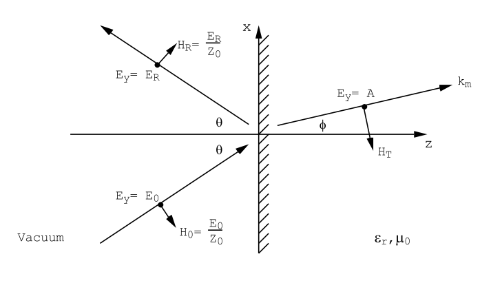
compared with Z₀= 377 Ohms for free space. This means that the electric field amplitude in the metal is very small compared with the electric field amplitude of the incident wave. At the interface between vacuum and the metal one must construct electric and magnetic field amplitudes so that the tangential components of \(\vec E\) and \(\vec H\) are continuous across the surface: the normal component of \(vec B\) is automatically continuous across the surface because the wave falls on the metal at normal incidence. These boundary conditions give

\[\begin{aligned}
&\text{E}_{0}+\text{E}_{\text{R}}=\text{A}\\
&\frac{1}{Z_{0}}\left(E_{0}-E_{R}\right)=\frac{A}{Z},
\end{aligned}\]

or

\[\text{E}_{0}-\text{E}_{\text{R}}=\frac{\text{Z}_{0} \text{A}}{\text{Z}}. \nonumber \]

The resulting wave amplitude at the metal surface, z=0, is

\[\text{A}=\frac{2 \text{ZE}_{0}}{\text{Z}+\text{Z}_{0}} \cong \frac{2 \text{Z}}{\text{Z}_{0}} \text{E}_{0} . \label{10.36}\]

The amplitude of the reflected wave is given by

\[\text{E}_{\text{R}}=\left(\frac{\text{Z}-\text{Z}_{0}}{\text{Z}+\text{Z}_{0}}\right) \text{E}_{0} , \nonumber \]

or

\[\frac{\text{E}_{\text{R}}}{\text{E}_{0}} \cong-1+\frac{2 \text{Z}}{\text{Z}_{0}}, \nonumber\]

because (Z/Z₀) ≪ 1.

Notice that for our example of copper at room temperature, and for a frequency of 1GHz, the magnitude of the reflected electric field amplitude is the same as the incident electric field amplitude to within ∼ 10⁻⁴ , but the reflected electric field is 180^◦ out of phase with the incident electric field so that the two fields cancel at the metal surface. The electric field in the metal is very small; approximately A= E₀/25000. On the other hand, the magnetic field amplitude at the metal surface is very nearly twice the magnetic field amplitude in the incident wave. In the metal at z=0

\[\text{H}_{\text{y}}=\frac{\text{A}}{\text{Z}}=\frac{2 \text{E}_{0}}{\text{Z}+\text{Z}_{0}} \cong 2 \frac{\text{E}_{0}}{\text{Z}_{0}} , \nonumber \]

whereas the magnetic field amplitude in the incident wave is given by E₀/Z₀.

One can speak of a perfectly conducting metal, one for which the conductivity approaches infinity. For such a perfectly conducting metal the electric field decays away in zero depth: a surface current sheet is set up that perfectly shields the metal from the electric field in the incident wave. The magnitude of the current sheet can be obtained by applying Stokes’ theorem to the relation \(\operatorname{curl}(\vec{\text{H}})=\vec{\text{J}}_{f}\) integrated over a small loop that spans the metal surface as shown in Figure (10.4.5). One has

\[\int int_{\text {Area}} \operatorname{curl}(\vec{\text{H}}) \cdot \vec{\text{d} \text{S}}=\int \int_{\text {Area}} \vec{\text{J}}_{f} \cdot \vec{\text{d} \text{S}}, \nonumber \]

where Area=\(\delta\)L. But from Stokes’ theorem

\[\oint_{C} \vec{\text{H}} \cdot \vec{\text{d} \text{L}}=\int \int_{A r e a} \vec{\text{J}}_{f} \cdot \vec{\text{dS}}=\text{J}_{\text{s}} \text{L} , \label{10.37}\]

Figure \(\PageIndex{5}\): Diagram to aid in the calculation of the surface current density that shields the interior of a perfectly conducting metal from incident electric and magnetic fields.

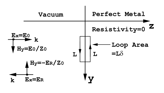
where J_s is the surface current density in Amps/m, and L is the length of the loop. Inside the metal H_y = 0 so from (10.37) one obtains

\[\text{J}_{\text{s}}=\text{H}_{\text{y}}(0), \label{10.38}\]

where H_y(0) is the magnetic field amplitude at the vacuum/metal interface, and H_y(0) = 2E₀/Z₀.

For a perfect metal the wave impedance approaches zero, Z = E_x/H_y and Z → 0, so that in this limit the electric field has a node at the metal surface. For a perfect metal the boundary condition on the electric field at the interface becomes

\[\text{E}_{\text{t}}=0, \nonumber \]

where Et is the tangential component of the electric field.

It is straight forward to calculate the absorption coefficient for a metal surface from Equation (\ref{10.35}) and from the amplitude A Equation (\ref{10.36}):

\[\alpha=\frac{<\text{S}_{\text{z}}(\text {metal at } z=0)>}{\text{S}_{\text{z}}(\text {incident})}=\frac{4 \text{c}}{\omega \text{Z}_{0}^{2}}|\text{Z}|^{2} \sqrt{\frac{\omega \sigma_{0} \mu_{0}}{2}} , \nonumber \]

or

\[\alpha=\frac{2 \omega}{\text{c}} \sqrt{\frac{2}{\sigma_{0} \omega \mu_{0}}}=\frac{2 \omega \delta}{\text{c}} ,\label{10.39}\]

Figure \(\PageIndex{6}\): An S-polarized plane wave incident at the angle θ on the plane interface between vacuum and an isotropic medium characterized by material parameters \(\epsilon_{\text{r}}\) and µ₀. The electric vector in the incident wave is perpendicular to the plane of incidence.

where \(\delta=\sqrt{\frac{2}{\omega \sigma_{0} \mu_{0}}}\) is the characteristic length for attenuation of the fields in the metal.