3.7: The Simple Dipole

As you may expect from the title of this section, this will be the most difficult and complicated section of this chapter so far. Our aim will be to calculate the field and potential surrounding a simple dipole.

A simple dipole is a system consisting of two charges, $+Q \text{ and }−Q$, separated by a distance $2L$. The dipole moment of this system is just $p = 2QL$. We’ll suppose that the dipole lies along the x-axis, with the negative charge at $x = −L$ and the positive charge at $x = +L$. See Figure $III$.5.

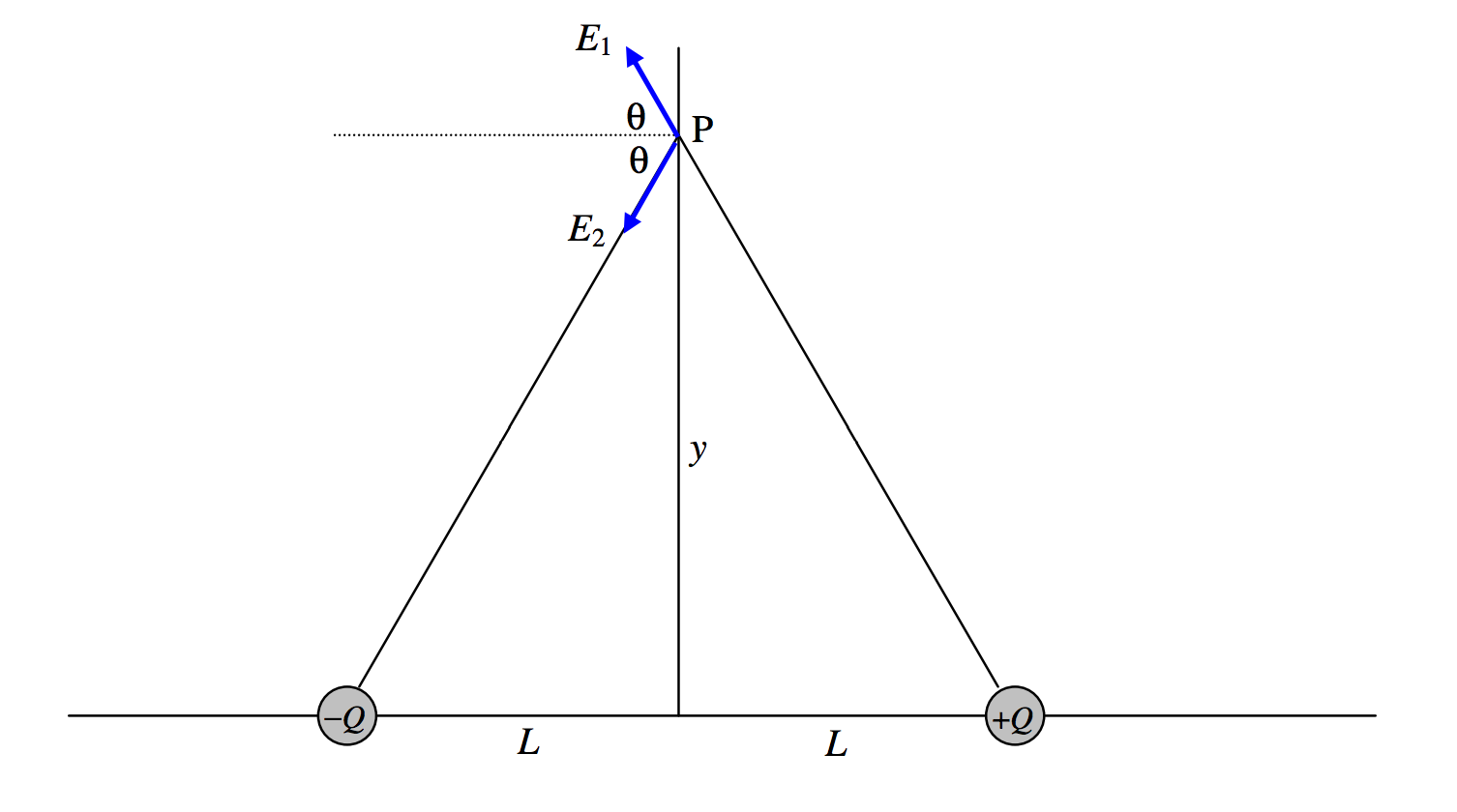
$\text{FIGURE III.5}$

Let us first calculate the electric field at a point P at a distance $y$ along the $y$-axis. It will be agreed, I think, that it is directed towards the left and is equal to

$$E_1 \cos \theta +E_2 \cos \theta,\text{ where }E_1=E_2=\dfrac{Q}{4\pi\epsilon_0 (L^2+y^2 )}\text{ and } \cos \theta = \dfrac{L}{(L^2+y^2)^{1/2}}.\nonumber$$

Therefore

$$E=\dfrac{2QL}{4\pi\epsilon_0(L^2+y^2)^{3/2}}=\dfrac{p}{4\pi\epsilon_0(L^2+y^2)^{3/2}}.\label{3.7.1}$$

For large $y$ this becomes

$$\label{3.7.2}E=\dfrac{p}{4\pi\epsilon_0y^3}.$$

That is, the field falls off as the cube of the distance.

To find the field on the $x$-axis, refer to Figure $III$.6.

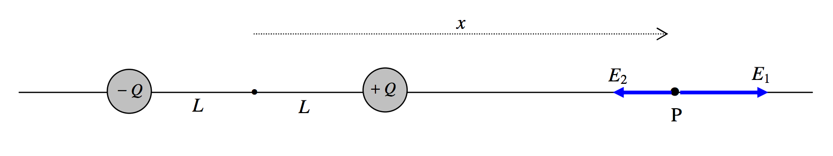
$\text{FIGURE III.6}$

It will be agreed, I think, that the field is directed towards the right and is equal to

$$\label{3.7.3}E=E_1-E_2=\dfrac{Q}{4\pi\epsilon_0} \left (\dfrac{1}{(x-L)^2}-\dfrac{1}{(x+L)^2}\right ).$$

This can be written $\dfrac{Q}{4\pi\epsilon_0x^2} \left (\dfrac{1}{(1-L/x)^2}-\dfrac{1}{(1+L/x)^2}\right )$, and on expansion of this by the binomial theorem, neglecting terms of order $(L / x)^2$ and smaller, we see that at large x the field is

$$\label{3.7.4}E=\dfrac{2p}{4\pi\epsilon_0x^3}.$$

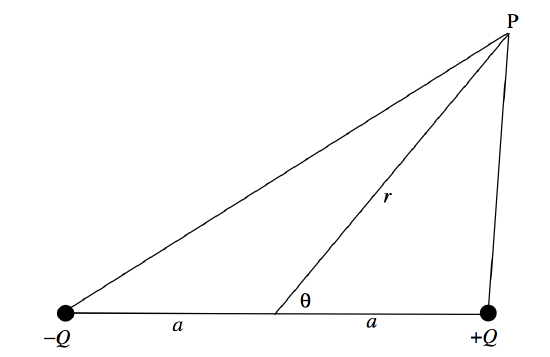
Now for the field at a point P that is neither on the axis ($x$-axis) nor the equator ($y$-axis) of the dipole. See Figure $III$.7.

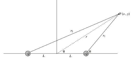
$\text{FIGURE III.7}$

It will probably be agreed that it would not be particularly difficult to write down expressions for the contributions to the field at P from each of the two charges in turn. The difficult part then begins; the two contributions to the field are in different and awkward directions, and adding them vectorially is going to be a bit of a headache.

It is much easier to calculate the potential at P, since the two contributions to the potential can be added as scalars. Then we can find the x- and y-components of the field by calculating $∂V / ∂x$ and $∂V/∂y$.

Thus

$$V=\dfrac{Q}{4\pi\epsilon_0}\left ( \dfrac{1}{\{(x-L)^2+y^2\}^{1/2}}-\dfrac{1}{\{(x+L)^2+y^2\}^{1/2}}\right ) . \label{3.7.5}$$

To start with I am going to investigate the potential and the field at a large distance from the dipole – though I shall return later to the near vicinity of it.

At large distances from a small dipole (see Figure $III$.8), we can write, $r^2=x^2+y^2$,

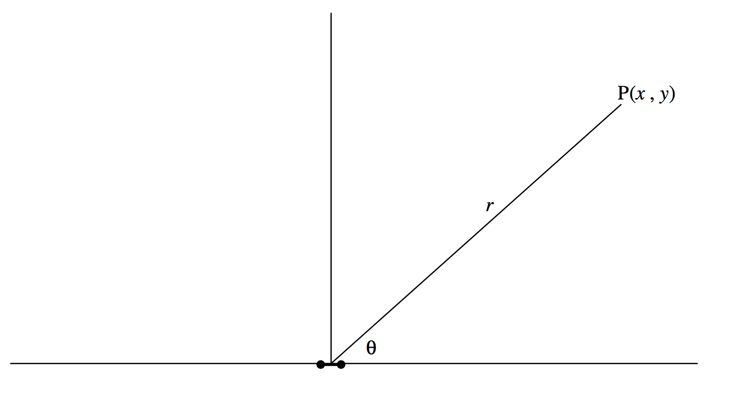
$\text{FIGURE III.8}$

and, with $L^2 << r^ 2$, the expression 3.7.5 for the potential at P becomes

$$V=\dfrac{Q}{4\pi\epsilon_0}\left ( \dfrac{1}{(r^2-2Lx)^{1/2}}-\dfrac{1}{(r^2+2Lx)^{1/2}}\right )=\dfrac{Q}{4\pi\epsilon_0 r}\left ( (1-2Lx/r^2)^{-1/2}-(1+2Lx/r^2)^{-1/2}\right ).\nonumber$$

When this is expanded by the binomial theorem we find, to order L/r , that the potential can be written in any of the following equivalent ways:

$$\label{3.7.6}V=\dfrac{2QLx}{4\pi\epsilon_0 r^3}=\dfrac{px}{4\pi\epsilon_0 r^3}=\dfrac{p\cos \theta}{4\pi\epsilon_0 r^2}=\dfrac{\textbf{p}\cdot \textbf{r}}{4\pi\epsilon_0 r^3}.$$

Thus the equipotentials are of the form

$$\label{3.7.7}r^2=c\cos \theta ,$$

where

$$\label{3.7.8}c=\dfrac{p}{4\pi\epsilon_0 V}.$$

Now, bearing in mind that $r^2+x^2+y^2$, we can differentiate $V=\dfrac{px}{4\pi\epsilon_0 r^3}$ with respect to $x$ and $y$ to find the $x$- and $y$-components of the field. Thus we find that

$$\label{3.7.9}E_x =\dfrac{p}{4\pi\epsilon_0}\left ( \dfrac{3x^2-r^2}{r^5}\right ) \text{ and }E_y=\dfrac{pxy}{4\pi\epsilon r^5}.$$

We can also use polar coordinates to find the radial and transverse components from $E_r=-\dfrac{∂V}{∂r}\text{ and }E_\theta = -\dfrac{1}{r}\dfrac{∂V}{∂\theta}\text{ together with }V=\dfrac{p\cos \theta}{4\pi\epsilon_0 r^2}$ to obtain

$$\label{3.7.10}E_r = \dfrac{2p\cos \theta}{4\pi\epsilon_0 r^3},\quad E_\theta = \dfrac{p\sin \theta }{4\pi\epsilon_0 r^3}\text{ and }E=\dfrac{p}{4\pi\epsilon_0 r^3}\sqrt{1+3 \cos^2 \theta}.$$

The angle that $\textbf{E}$ makes with the axis of the dipole at the point $(r, θ)$ is $θ + \tan^{-1}\dfrac{1}{2}\tan \theta$.

For those who enjoy vector calculus, we can also say $\textbf{E}=-\dfrac{1}{4\pi\epsilon_0}\nabla \left ( \dfrac{\textbf{p}\cdot \textbf{r}}{r^3}\right )$, from which, after a little algebra and quite a lot of vector calculus, we find

$$\label{3.7.11}\textbf{E}=\dfrac{1}{4\pi\epsilon_0}\left ( \dfrac{3(\textbf{p}\cdot \textbf{r})\textbf{r}}{r^5}-\dfrac{\textbf{p}}{r^3}\right ).$$

This equation contains all the information that we are likely to want, but I expect most readers will prefer the more explicit rectangular and polar forms of equations $\ref{3.7.9}$ and $\ref{3.7.10}$.

Equation $\ref{3.7.7}$ gives the equation to the equipotentials. The equation to the lines of force can be found as follows. Referring to Figure $III$.9, we see that the differential equation to the lines of force is

$\text{FIGURE III.9}$

$$\label{3.7.12}r\dfrac{d\theta}{dr}=\dfrac{E_\theta}{E_r}=\dfrac{\sin \theta}{2\cos \theta}=\dfrac{1}{2}\tan \theta ,$$

which, upon integration, becomes

$$\label{3.7.13}r=a\sin^2 \theta .$$

Note that the equations $r^2= c\cos θ$ (for the equipotentials) and $r= a \sin^2 \theta$ (for the lines of force) are orthogonal trajectories, and either can be derived from the other. Thus, given that the differential equation to the lines of force is $r\dfrac{d\theta}{dr}= \dfrac{1}{2}\tan \theta$ with solution $r=a\sin^2 \theta$, the differential equation to the orthogonal trajectories (i.e. the equipotentials) is $-\dfrac{1}{r}\dfrac{dr}{d\theta}=\dfrac{1}{2}\tan \theta$, with solution $r^2=c\cos \theta$.

In Figure $III$.10, there is supposed to be a tiny dipole situated at the origin. The unit of length is $L$, half the length of the dipole. I have drawn eight electric field lines (continuous), corresponding to a = 25, 50, 100, 200, 400, 800, 1600, 3200. If r is expressed in units of $L$, and if $V$ is expressed in units of $\dfrac{Q}{4\pi\epsilon_0 L}$, the equations $\ref{3.7.7}$ and $\ref{3.7.8}$ for the equipotentials can be written , $r=\sqrt{\dfrac{2\cos \theta}{V}}$, and I have drawn seven equipotentials (dashed) for $V$ = 0.0001, 0.0002, 0.0004, 0.0008, 0.0016, 0.0032, 0.0064. It will be noticed from Equation $\ref{3.7.9a}$, and is also evident from Figure $III$.10, that $E_x$ is zero for $\theta = 54^\circ \, 44'$.

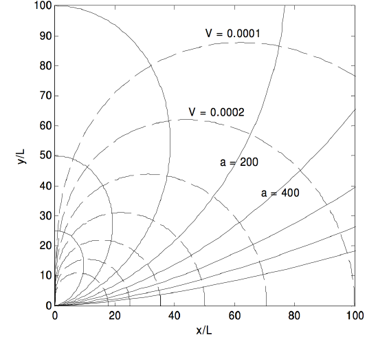
$\text{FIGURE III.10}$

At the end of this chapter I append a (geophysical) exercise in the geometry of the field at a large distance from a small dipole.

Equipotentials near to the dipole

These, then, are the field lines and equipotentials at a large distance from the dipole. We arrived at these equations and graphs by expanding Equation $\ref{3.7.5}$ binomially, and neglecting terms of higher order than $L/r$. We now look near to the dipole, where we cannot make such an approximation. Refer to Figure $III$.7.

We can write Equation $\ref{3.7.5}$ as

$$\label{3.7.14}V(x,y)=\dfrac{Q}{4\pi\epsilon_0}\left ( \dfrac{1}{r_1}-\dfrac{1}{r_2}\right ),$$

where $r_1^2=(x-L)^2+y^2 \text{ and }r_2^2=(x+L)^2+y^2$. If, as before, we express distances in terms of $L$ and $V$ in units of $\dfrac{Q}{4\pi\epsilon_0 L}$, the expression for the potential becomes

$$\label{3.7.15}V(x,y)\dfrac{1}{r_1}-\dfrac{1}{r_2},$$

where $r_1^2=(x+1)^2+y^2 \text{ and }r_2^2=(x-1)^2+y^2$.

One way to plot the equipotentials would be to calculate $L$ for a whole grid of $(x , y)$ values and then use a contour plotting routine to draw the equipotentials. My computing skills are not up to this, so I’m going to see if we can find some way of plotting the equipotentials directly.

I present two methods. In the first method I use Equation $\ref{3.7.15}$ and endeavour to manipulate it so that I can calculate $y$ as a function of $x$ and $L$. The second method was shown to me by J. Visvanathan of Chennai, India. We’ll do both, and then compare them.

First Method.

To anticipate, we are going to need the following:

$$\begin{align} &r_1^2r_2^2=(x^2+y^2+1)^2-4x^2=B^2-A,\label{3.7.16} \\ &r_1^2+r_2^2 = 2(x^2+y^2+1)=2B,\label{3.7.17}\\ \text{and} \quad &r_1^4+r_2^4=2[(x^2+y^2+1)^2+4x^2]=2(B^2+A),\label{3.7.18} \\ \text{where}\quad \,&A=4x^2 \label{3.7.19} \\ \text{and}\quad &B=x^2+y^2+1 \label{3.7.20} \\ \end{align}$$

Now Equation $\ref{3.7.15}$ is $r_1r_2 V=r_2-r_1$. In order to extract $y$ it is necessary to square this twice, so that $r_1 \text{ and }r_2$ appear only as $r_1^2 \text{ and }r_2^2$. After some algebra, we obtain

$$\label{3.7.21}r_1^2r_2^2 [2-V^4r_1^2r_2^2+2V^2(r_1^2 +r_2^2)]=r_1^4+r_2^4.$$

Upon substitution of equations $\ref{3.7.16}$,17,18, for which we are well prepared, we find for the equation to the equipotentials an equation which, after some algebra, can be written as a quartic equation in B:

$$\begin{align}&a_0+a_1B+a_2B^2+a_3B^3+a_4B^4=0 \label{3.7.22} \\ \text{where}\quad &a_0=A(4+V^4A), \label{3.7.23} \\ &a_1=4V^2A, \label{3.7.24} \\ &a_2 = -2V^2A,\label{3.7.25} \\ &a_3=-4V^2,\label{3.7.26} \\ \text{and} \quad &a_4 = V^4 .\label{3.7.27} \\ \end{align}$$

The algorithm will be as follows: For a given $V$ and $x$, calculate the quartic coefficients from equations $\ref{3.7.23}$-$\ref{3.7.27}$. Solve the quartic Equation $\ref{3.7.22}$ for B. Calculate y from Equation $\ref{3.7.20}$. My attempt to do this is shown in Figure $III$.11. The dipole is supposed to have a negative charge at (−1 , 0) and a positive charge at (+1 , 0). The equipotentials are drawn for $V$ = 0.05, 0.10, 0.20, 0.40, 0.80.

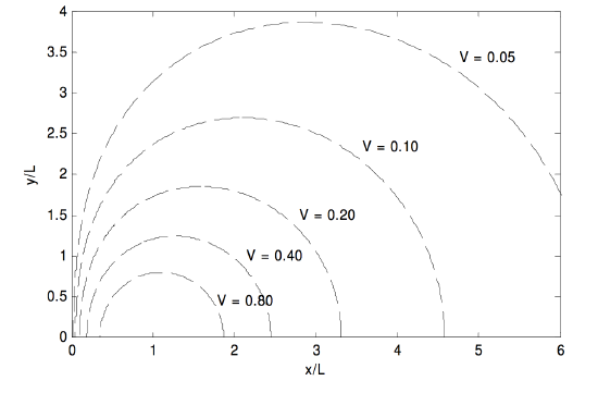
$\text{FIGURE III.11}$

Second method (J. Visvanathan).

In this method, we work in polar coordinates, but instead of using the coordinates $(r,θ)$, in which the origin, or pole, of the polar coordinate system is at the center of the dipole (see Figure $III$.7), we use the coordinates $(r_1, \phi)$ with origin at the positive charge.

From the triangle, we see that

$$r_2^2=r_1^2+4L^2 +4Lr_1\cos \phi .\label{3.7.28}$$

For future reference we note that

$$\dfrac{∂r_2}{∂r_1}=\dfrac{r_1 +2L\cos \phi }{r_2}.\label{3.7.29}$$

Provided that distances are expressed in units of $L$, these equations become

$$\label{3.7.30}r_2^2=r_1^2 + 4r_1 \cos \phi + 4,$$

$$\dfrac{∂r_2}{∂r_1}=\dfrac{r_1+2\cos \phi}{r_2}.\label{3.7.31}$$

If, in addition, electrical potential is expressed in units of $\dfrac{Q}{4\pi\epsilon_0 L}$, the potential at P is given, as before (Equation $\ref{3.7.15}$), by

$$\label{3.7.32}V(r_1,\phi )=\dfrac{1}{r_1}-\dfrac{1}{r_2}.$$

bearing in mind that $r_2$ is given by Equation $\ref{3.7.31}$.

By differentiation with respect to $r_1$, we have

$$\label{3.7.34}f'(r_1)=-\dfrac{1}{r_1^2}+\dfrac{1}{r_2^2}\dfrac{∂r_2}{∂r_1}=-\dfrac{1}{r_1^2}+\dfrac{r_1+2\cos \phi}{r_2^3},$$

and we are all set to begin a Newton-Raphson iteration: $r_1=r_1-f/f'$. Having obained $r_1$, we can then obtain the $(x,\, y)$ coordinates from $x = 1 + r_1 \cos φ \text{ and }y = r_1 \sin φ$.

I tried this method and I got exactly the same result as by the first method and as shown in Figure $III$.11.

So which method do we prefer? Well, anyone who has worked through in detail the derivations of equations $\ref{3.7.16}$ -$\ref{3.7.27}$, and has then tried to program them for a computer, will agree that the first method is very laborious and cumbersome. By comparison Visvanathan’s method is much easier both to derive and to program. On the other hand, one small point in favor of the first method is that it involves no trigonometric functions, and so the numerical computation is potentially faster than the second method in which a trigonometric function is calculated at each iteration of the Newton-Raphson process. In truth, though, a modern computer will perform the calculation by either method apparently instantaneously, so that small advantage is hardly relevant.

So far, we have managed to draw the equipotentials near to the dipole. The lines of force are orthogonal to the equipotentials. After I tried several methods with only partial success, I am grateful to Dr Visvanathan who pointed out to me what ought to have been the “obvious” method, namely to use Equation $\ref{3.7.12}$, which, in our $(r_1,\phi)$ coordinate system based on the positive charge, is $r_1\dfrac{d\phi}{dr_1}=\dfrac{E_\phi}{E_{r_1}}$, just as we did for the large distance, small dipole, approximation. In this case, the potential is given by equations $\ref{3.7.30}$ and $\ref{3.7.32}$. (Recall that in these equations, distances are expressed in units of L and the potential in units of $\dfrac{Q}{4\pi\epsilon_0 L}$.) The radial and transverse components of the field are given by $E_{r_1}=-\dfrac{∂V}{∂{r_1}}\text{ and } E_\phi=-\dfrac{1}{r_1}\dfrac{∂V}{∂\phi}$, which result in

$$E_{r_1}=\dfrac{1}{r_1^2}-\dfrac{r_1+2\cos \phi }{r_2^3}\label{3.7.35}$$

and

$$E_\phi = \dfrac{2\sin \phi}{r_2^3}.\label{3.7.36}$$

Here, the field is expressed in units of $\dfrac{Q}{4\pi\epsilon_0L^2}$, although that hardly matters, since we are interested only in the ratio. On applying $r_1\dfrac{d\phi}{dr}=\dfrac{E_\phi}{E_{r_1}}$ to these field components we obtain the following differential equation to the lines of force:

$$d\phi = \dfrac{2r_1\sin \phi}{(r_1^2+4+4r_1\cos \phi)^{3/2}-r_1^2(r_1+2\cos \phi)}dr_1.\label{3.7.37}$$

Thus one can start with some initial $φ_0$ and small $r_2$ and increase $r_1$ successively by small increments, calculating a new φ each time. The results are shown in Figure $III$.12, in which the equipotentials are drawn for the same values as in Figure $III$.11, and the initial angles for the lines of force are 30º, 60º, 90º, 120º, 150º.

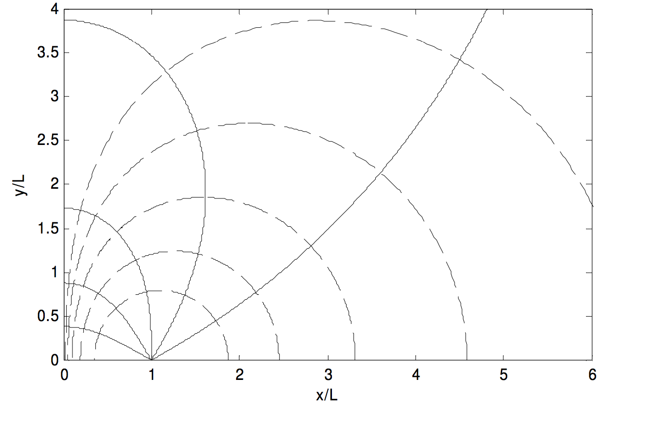
$\text{FIGURE III.12}$

Before we leave this section, here is yet another method of calculating the potential near to a dipole, for those who are familiar with Legendre polynomials.

The potential at P is given by

$$\nonumber \begin{align}4\pi\epsilon_0V&=Q \left [ \dfrac{1}{(a^2+r^2-2ar\cos \theta )^{1/2}}-\dfrac{1}{(a^2+r^2+2ar\cos \theta )^{1/2}}\right ] \\ \nonumber &=\dfrac{Q}{a} \left [ \dfrac{1}{(1-2\rho \cos \theta + \rho^2)^{1/2}}-\dfrac{1}{1+2\rho \cos \theta + \rho^2)^{1/2}}\right ] \\ \end{align}$$

where $\rho = r/a$.

It is well known (to those who are familiar with Legendre polynomials!) that

$$\nonumber (1-2\rho\cos \theta +\rho^2)^{-1/2}=P_0(\cos \theta)+P_1(\cos \theta)\rho +P_2(\cos \theta )\rho^2+P_3(x)\rho^3+...$$

where the $P_n$ are the Legendre polynomials. Thus the potential can be calculated as a series expansion. Those who are unfamiliar with the Legendre polynomials can find something about them in my notes on celestial mechanics www.astro.uvic.ca/~tatum/celmechs/celm1.pdf