1.2: Forces and the Measurement and Nature of Electromagnetic Fields

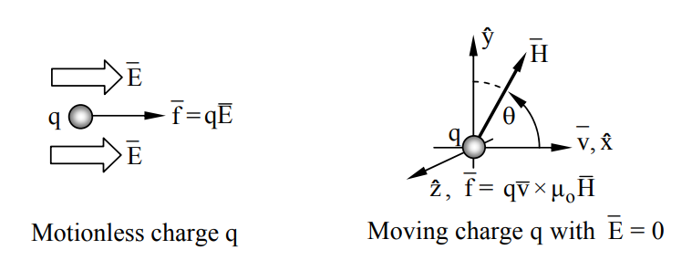
Electric fields \(\overline E\) and magnetic fields \(\overline H\) are manifest only by the forces they exert on free or bound electric charges q [Coulombs]. These forces are completely characterized by the Lorentz force law:

\[\overline{\mathrm{f}}[\mathrm{N}]=\mathrm{q}\left(\overline{\mathrm{E}}+\overline{\mathrm{v}} \times \mu_{\mathrm{o}} \overline{\mathrm{H}}\right) \quad \text { (Lorentz force law) }\]

Thus we can define electric field \(\overline E\) (volts/meter) in terms of the observable force vector \(\overline f\):

\[\overline{\mathrm{E}}[\mathrm{v} / \mathrm{m}]=\overline{\mathrm{f}} / \mathrm{q}\quad \text { (electric field) }\]

for the special case of a charge q with velocity \(\overline v\) = 0 .

Similarly we can define magnetic field \(\overline{\mathrm{H}}\left[\mathrm{A} \mathrm{m}^{-1}\right]\) in terms of the observed force vector \(\overline f\) given by the Lorentz force equation when \(\overline{\mathrm{E}}\)= 0 ; \(\overline{\mathrm{H}}\) can be sensed only by charges in motion relative to the observer. Although a single measurement of force on a motionless charge suffices to determine \(\overline{\mathrm{E}}\), measurements of two charge velocity vectors \(\overline v\) or current directions \(\overline{\mathrm{I}}\) are required to determine \(\overline{\mathrm{H}}\). For example, the arbitrary test charge velocity vector \(\hat{x} \mathrm{v}_{1} \text { yields } \mathrm{f}_{1}= \mathrm{q} \mu_{\mathrm{o}} \mathrm{v}_{1} \mathrm{H} \sin \theta\), where \(\theta\) is the angle between \(\overline{\mathrm{v}}\) and \(\overline{\mathrm{H}}\) in the \(\hat{x}-\hat{y}\) plane (see Figure 1.2.1). The unit vector \(\hat{y}\) is defined as being in the observed direction \(\overline{\mathrm{f}}_{1} \times \overline{\mathrm{v}}_{1}\) where \(\overline{\mathrm{f}}_{1}\) defines the \(\hat{z}\) axis. A second measurement with the test charge velocity vector \(\hat{y} \mathrm{v}_{2} \text { yields } \mathrm{f}_{2}=\mathrm{q} \mu_{\mathrm{o}} \mathrm{v}_{2} \mathrm{H} \cos \theta\). If \(\mathbf{v}_{1}=v_{2}\) then the force ratio \(\mathrm{f}_{\mathrm{l}} / \mathrm{f}_{2}=\tan \theta\), yielding \(\theta\) within the \(\hat{x}-\hat{y}\) plane, plus the value of \(\mathrm{H}: \mathrm{H}=\mathrm{f}_{\mathrm{I}} /\left(\mathrm{q} \mu_{\mathrm{n}} \mathrm{v}_{\mathrm{I}} \sin \theta\right)\). There is no other physical method for detecting or measuring static electric or magnetic fields; we can only measure the forces on charges or on charged bodies, or measure the consequences of that force, e.g., by measuring the resulting currents.

Figure \(\PageIndex{1}\): Measurement of electric and magnetic fields using charges.

It is helpful to have a simple physical picture of how fields behave so that their form and behavior can be guessed or approximately understood without recourse to mathematical solutions. Such physical pictures can be useful even if they are completely unrelated to reality, provided that they predict all observations in a simple way. Since the Lorentz force law plus Maxwell’s equations explain essentially all non-relativistic and non-quantum electromagnetic behavior in a simple way using the fields \(\overline E\) and \(\overline H\), we need only to ascertain how \(\overline E\) and \(\overline H\) behave given a particular distribution of stationary or moving charges q.

First consider static distributions of charge. Electric field lines are parallel to \(\overline E\), and the strength of \(\overline E\) is proportional to the density of those field lines. Electric field lines begin on positive charges and terminate on negative ones, and the more charge there is, the more field lines there are. Field strength is proportional to lines per square meter. These lines pull on those charges to which they are attached, whether positive or negative, much as would a rubber band. Like rubber bands, they would also like to take the shortest path between two points, except that they also tend to repel their neighbors laterally, as do the charges to which they are attached.

Figure \(\PageIndex{2}\): Electric field lines between two conducting cylinders.

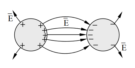
Figure 1.2.2 illustrates the results of this mutual field-line repulsion, even as they pull opposite charges on conducting cylinders toward one another. Later we shall see that such electric field lines are always perpendicular to perfectly conducting surfaces. Although these lines are illustrated as discrete, they actually are a continuum, even if only two charges are involved.

The same intuition applies to magnetic field lines \(\overline H\). For example, Figure 1.2.2 would apply if the two cylinders corresponded instead to the north (+) and south (-) poles of a magnet, and if \(\overline E\) became \(\overline H\), although \(\overline H\) need not emerge perfectly perpendicular to the magnet surface. In this case too the field lines would physically pull the two magnet poles toward one another. Both electric and magnetic motors can be driven using either the attractive force along field lines or the lateral repulsive force between lines, depending on motor design, as discussed later.

Another intuitive picture applies to time-dependent electromagnetic waves, where distributions of position-dependent electric and magnetic fields at right angles propagate as plane waves in the direction \(\overline E\) × \(\overline H\) much like a rigid body at the speed of light c, ~3×10⁸ m/s. Because electromagnetic waves can superimpose, it can be shown that any distribution of electric and magnetic fields can be considered merely as the superposition of such plane waves. Such plane waves are introduced in Section 2.2. If we examine such superpositions on spatial scales small compared to a wavelength, both the electric and magnetic fields behave much as they would in the static case.

Example \(\PageIndex{A}\)

A typical old vacuum tube accelerates electrons in a ~10⁴ v m^-1 electric field. What is the resulting electron velocity v(t) if it starts from rest? How long (\(\tau\)) does it take the electron to transit the 1-cm tube?

Solution

Force

\[f = ma = qE,\]

and so

\[v = at = \dfrac{qEt}{m} ≅ \dfrac{1.6×10^{-19} ×10 ^4 t}{9.1×10^{-28}} ≅ 1.8×10^{12}\, t [m\, s^{-1}].\]

Obviously \(v\) cannot exceed the speed of light c, ~3×10⁸ m/s. In this text we deal only with non-relativistic electrons traveling much slower than c. Distance traveled = d = a\(\tau\)² /2 = 0.01, so the transit time

\(\tau\) = (2d/a)^0.5 = (2dm/qE)^0.5 ≅ [2×0.01×9.1×10^-28 /(1.6×10^-19 ×10⁴ )]0.5 ≅ 1.1×10^-7 seconds.

This slow transit limited most vacuum tubes to signal frequencies below several megahertz, although smaller gaps and higher voltages have enabled simple tubes to reach 100 MHz and higher. The microscopic gaps of semiconductors can eliminate transit time as an issue for most applications below 1 GHz; other phenomena often determine the frequency range instead.