3.2: Inductors and Transformers

Solenoidal inductors

All currents in devices produce magnetic fields that store magnetic energy and therefore contribute inductance to a degree that depends on frequency. When two circuit branches share magnetic fields, each will typically induce a voltage in the other, thus coupling the branches so they form a transformer, as discussed in Section 3.2.4.

Inductors are two-terminal passive devices specifically designed to store magnetic energy, particularly at frequencies below some design-dependent upper limit. One simple geometry is shown in Figure 3.2.1 in which current i(t) flows in a loop through two perfectly conducting parallel plates of width W and length D, spaced d apart, and short-circuited at one end.

Figure \(\PageIndex{1}\): Parallel-plate inductor.

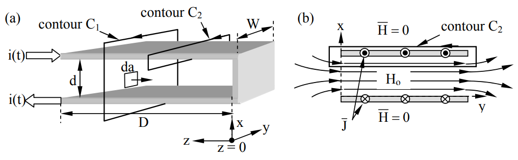
To find the magnetic field from the currents we can use the integral form of Ampere’s law, which links the variables \(\overline H\) and \(\overline J\) :

\[ \oint_{\text{C}} \overline{\text{H}} \bullet \text{d} \overline{\text{s}}=\int \int_{\text{A}}(\overline{\text{J}}+\partial \overline{\text{D}} / \partial \text{t}) \cdot \text{d} \overline{\text{a}}\]

The contour C₁ around both currents in Figure 3.2.1 encircles zero net current, and (3.2.1) says the contour integral of \(\overline H\) around zero net current must be zero in the static case. Contour C₂ encircles only the current i(t), so the contour integral of \(\overline H\) around any C₂ in the right-hand sense equals i(t) for the static case. The values of these two contour integrals are consistent with zero magnetic field outside the pair of plates and a constant field \(\overline{\text{H}}=\text{H}_{\text{o}} \hat{y}\) between them, although a uniform magnetic field could be superimposed everywhere without altering those integrals. Since such a uniform field would not have the same symmetry as this device, such a field would have to be generated elsewhere. These integrals are also exactly consistent with fringing fields at the edges of the plate, as illustrated in Figure 3.2.1(b) in the x-y plane for z > 0. Fringing fields can usually be neglected if the plate separation d is much less than the plate width W.

It follows that:

\[\oint_{\text{C} 2} \overline{\text{H}} \bullet \text{d} \overline{\text{s}}=\text{i}(\text{t})=\text{H}_{\text{o}} \text{W} \]

\[\overline{\text{H}}=\hat{y} \text{H}_{\text{o}}=\hat{y} \text{i}(\text{t}) / \text{W}\left[\text{A} \text{m}^{-1}\right] \qquad\qquad\quad(\overline{\text{H}} \text { between the plates }) \]

and \(\overline H\) ≅ 0 elsewhere.

Figure \(\PageIndex{2}\): Voltages induced on a parallel-plate inductor.

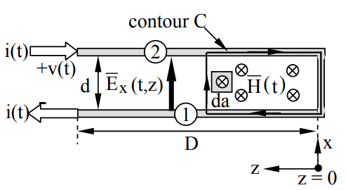
The voltage v(t) across the terminals of the inductor illustrated in Figures 3.2.1 and 3.2.2 can be found using the integral form of Faraday’s law and (3.2.3):

\[\oint_{\text{C}} \overline{\text{E}} \bullet \text{d} \overline{\text{s}}=-\frac{\partial}{\partial \text{t}} \int \int_{\text{A}} \mu \overline{\text{H}} \bullet \text{d} \overline{\text{a}}=-\frac{\mu \text{D} \text{d}}{\text{W}} \frac{\text{d} \text{i}(\text{t})}{\text{dt}}=\int_{1}^{2} \text{E}_{\text{x}}(\text{t}, \text{z}) \text{d} \text{x}=-\text{v}(\text{t}, \text{z})\]

where z = D at the inductor terminals. Note that when we integrate \(\overline E\) around contour C there is zero contribution along the path inside the perfect conductor; the non-zero portion is restricted to the illustrated path 1-2. Therefore:

\[\text{v}(\text{t})=\frac{\mu \text{Dd}}{\text{W}} \frac{\text{di}(\text{t})}{\text{dt}}=\text{L} \frac{\text{di}(\text{t})}{\text{dt}}\]

where (3.2.5) defines the inductance L [Henries] of any inductor. Therefore L₁ for a single-turn current loop having length W >> d and area A = Dd is:

\[\text{L}_{1}=\frac{\mu \text{Dd}}{\text{W}}=\frac{\mu \text{A}}{\text{W}}\ [\text{H}] \qquad \qquad \quad \text { (single-turn wide inductor) } \]

To simplify these equations we define magnetic flux \(\psi_{\text{m}}\) as⁸ :

\[ \psi_{\text{m}}=\int \int_{\text{A}} \mu \overline{\text{H}} \bullet \text{d} \overline{\text{a}} \ [\text{Webers}=\text{Vs}]\]

Then Equations (3.2.4) and (3.2.7) become:

\[ \text{v}(\text{t})=\text{d} \psi_{\text{m}}(\text{t}) / \text{d} \text{t}\]

\[\psi_{\text{m}}(\text{t})=\text{L} \ \text{i}(\text{t}) \qquad \qquad \quad \text{(single-turn inductor) } \]

Since we assumed fringing fields could be neglected because W >> d, large single-turn inductors require very large structures. The standard approach to increasing inductance L in a limited volume is instead to use multi-turn coils as illustrated in Figure 3.2.3.

Figure \(\PageIndex{3}\): N-turn inductor: (a) solenoid, (b) toroid.

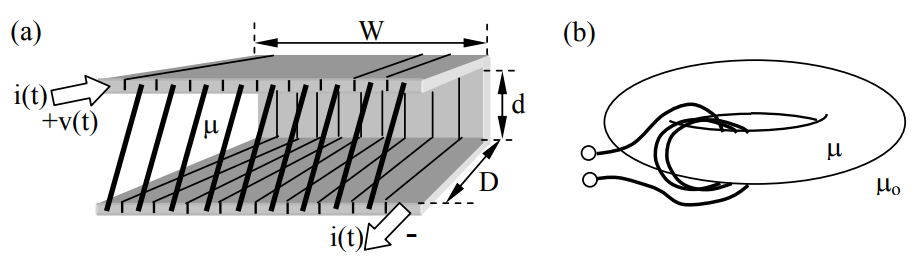
The N-turn coil of Figure 3.2.3 duplicates the current flow geometry illustrated in Figures 3.2.1 and 3.2.2, but with N times the intensity (A m^-1) for the same terminal current i(t), and therefore the magnetic field H_o and flux \(\psi_{\mathrm{m}}\) are also N times stronger than before. At the same time the voltage induced in each turn is proportional to the flux \( \psi_{\text{m}}\) through it, which is now N times greater than for a single-turn coil (\(\psi_{\text{m}} \)= NiμA/W), and the total voltage across the inductor is the sum of the voltages across the N turns. Therefore, provided that W >> d, the total voltage across an N-turn inductor is N² times its one-turn value, and the inductance L_N of an N-turn coil is also N² greater than L₁ for a one-turn coil:

\[\text{v}(\text{t})=\text{L}_{\text{N}} \frac{\text{di}(\text{t})}{\text{dt}}=\text{N}^{2} \text{L}_{1} \frac{\text{di}(\text{t})}{\text{dt}} \]

\[ \text{L}_{\text{N}}=\text{N}^{2} \frac{\mu \text{A}}{\text{W}} \ [H] \qquad\qquad\quad \text { (N-turn solenoidal inductor) }\]

where A is the coil area and W is its length; \(W>>\sqrt{A}>d\).

Equation (3.2.11) also applies to cylindrical coils having W >> d, which is the most common form of inductor. To achieve large values of N the turns of wire can be wound on top of each other with little adverse effect; (3.2.11) still applies.

These expressions can also be simplified by defining magnetic flux linkage Λ as the magnetic flux \(\psi_{\text{m}} \) (3.2.7) linked by N turns of the current i, where:

\[ \Lambda=\text{N} \psi_{\text{m}}=\text{N}(\text{Ni} \mu \text{A} / \text{W})=\left(\text{N}^{2} \mu \text{A} / \text{W}\right) \text{i}=\text{Li} \qquad\qquad\quad \text { (flux linkage) }\]

This equation Λ = Li is dual to the expression Q = Cv for capacitors. We can use (3.2.5) and (3.2.12) to express the voltage v across N turns of a coil as:

\[\text{v}=\text{L} \text{di} / \text{dt}=\text{d} \Lambda / \text{dt} \qquad\qquad\quad \text { (any coil linking magnetic flux } \Lambda \text { ) } \]

The net inductance L of two inductors L₁ and L₂ in series or parallel is related to L₁ and L₂ in the same way two connected resistors are related:

\[\text{L}=\text{L}_{1}+\text{L}_{2} \qquad\qquad\quad \text { (series combination) } \]

\[\text{L}^{-1}=\text{L}_{1}^{-1}+\text{L}_{2}^{-1} \qquad \qquad \quad \text { (parallel combination) } \]

For example, two inductors in series convey the same current i but the total voltage across the pair is the sum of the voltages across each – so the inductances add.

Example \(\PageIndex{A}\)

Design a 100-Henry air-wound inductor.

Solution

Equation (3.2.11) says L = N² μA/W, so N and the form factor A/W must be chosen. Since A = \(\pi\)r² is the area of a cylindrical inductor of radius r, then W = 4r implies L = N² μ\(\pi\)r/4. Although tiny inductors (small r) can be achieved with a large number of turns N, N is limited by the ratio of the cross-sectional areas of the coil rW and of the wire \(\pi\)r_w² , and is N ≅ r² /r_w² . N is further limited if we want the resistive impedance R << jωL. If ω_min is the lowest frequency of interest, then we want R ≅ ω_minL/100 = d/(σ\(\pi\)r_w²) [see (3.1.5)], where the wire length d ≅ 2\(\pi\)rN. These constraints eventually yield the desired values for r and N that yield the smallest inductor. Example 3.2B carries these issues further.

Toroidal inductors

The prior discussion assumed μ filled all space. If μ is restricted to the interior of a solenoid, L is diminished significantly, but coils wound on a high-μ toroid, a donut-shaped structure as illustrated in Figure 3.2.3(b), yield the full benefit of high values for μ. Typical values of μ are ~5000 to 180,000 for iron, and up to ~10⁶ for special materials.

Coils wound on high-permeability toroids exhibit significantly less flux leakage than solenoids. Consider the boundary between air and a high-permeability material (μ/μ_o >>1), as illustrated in Figure 3.2.4.

Figure \(\PageIndex{4}\): Magnetic fields at high-permeability boundaries.

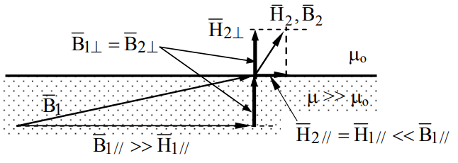
The degree to which \(\overline B\) is parallel or perpendicular to the illustrated boundary has been diminished substantially for the purpose of clarity. The boundary conditions are that both \(\overline{\text{B}}_{\perp}\) and \(\overline{\text{H}}_{//} \) are continuous across any interface (2.6.5, 2.6.11). Since \(\overline{\text{B}}=\mu \overline{\text{H}}\) in the permeable core and \( \overline{\text{B}}=\mu_{\text{o}} \overline{\text{H}}\) in air, and since \(\overline{\text{H}}_{//} \) is continuous across the boundary, therefore \(\overline{\text{B}}_{//} \) changes across the boundary by the large factor μ/μ_ο. In contrast, \(\overline{\text{B}}_{\perp}\) is the same on both sides. Therefore, as suggested in Figure 3.2.4, \( \overline{\text{B}}_{2}\) in air is nearly perpendicular to the boundary because \(\overline{\mathrm{H}}_{/ /}\), and therefore \(\overline{\text{B}}_{2 / /} \), is so very small; note that the figure has been scaled so that the arrows representing \(\overline{\mathrm{H}}_{2} \) and \(\overline{\text{B}}_{2} \) have the same length when μ = μ₀.

Figure \(\PageIndex{5}\): Toroidal inductor.

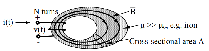
In contrast, \( \overline{\text{B}}_{1}\) is nearly parallel to the boundary and is therefore largely trapped there, even if that boundary curves, as shown for a toroid in Figure 3.2.5. The reason magnetic flux is largely trapped within high-μ materials is also closely related to the reason current is trapped within high-σ wires, as described in Section 4.3.

The inductance of a toroidal inductor is simply related to the linked magnetic flux Λ by (3.2.12) and (3.2.7):

\[ \text{L}=\frac{\Lambda}{\text{i}}=\frac{\mu \text{N} \int \int_{\text{A}} \overline{\text{H}} \bullet \text{d} \overline{\text{a}}}{\text{i}} \qquad\qquad\qquad \text { (toroidal inductor) }\]

where A is any cross-sectional area of the toroid.

Computing \(\overline H \) is easier if the toroid is circular and has a constant cross-section A which is small compared to the major radius R so that \( \text{R}>>\sqrt{\text{A}}\). From Ampere’s law we learn that the integral of \(\overline H \) around the 2\(\pi\)R circumference of this toroid is:

\[\oint_{\text{C}} \overline{\text{H}} \bullet \text{d} \overline{\text{s}} \cong 2 \pi \text{RH} \cong \text{Ni} \]

where the only linked current is i(t) flowing through the N turns of wire threading the toroid. Equation (3.2.17) yields H ≅ Ni/2\(\pi\)R and (3.2.16) relates H to L. Therefore the inductance L of such a toroid found from (3.2.16) and (3.2.17) is:

\[\text{L} \cong \frac{\mu \text{NA}}{\text{i}} \frac{\text{Ni}}{2 \pi \text{R}}=\frac{\mu \text{N}^{2} \text{A}}{2 \pi \text{R}} \ [\text { Henries }] \qquad\qquad\qquad(\text { toroidal inductor }) \]

The inductance is proportional to μ, N² , and cross-sectional area A, but declines as the toroid major radius R increases. The most compact large-L toroids are therefore fat (large A) with almost no hole in the middle (small R); the hole size is determined by N (made as large as possible) and the wire diameter (made small). The maximum acceptable series resistance of the inductor limits N and the wire diameter; for a given wire mass [kg] this resistance is proportional to N² .

Figure \(\PageIndex{6}\): Toroidal inductor with a small gap.

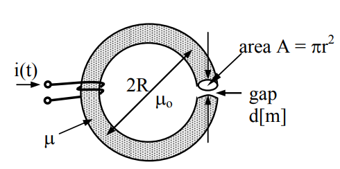
The inductance of a high-permeability toroid is strongly reduced if even a small gap of width d exists in the magnetic path, as shown in Figure 3.2.6. The inductance L of a toroid with a gap of width d can be found using (3.2.16), but first we must find the magnitude of H_μ within the toroid. Again we can use the integral form of Ampere’s law for a closed contour along the axis of the toroid, encircling the hole.

\[ \oint_{\text{C}} \overline{\text{H}} \bullet \text{d} \overline{\text{s}} \cong(2 \pi \text{R}-\text{d}) \text{H}_{\mu}+\text{H}_{\text{g}} \text{d} \cong \text{Ni}\]

where H_g is the magnitude of H within the gap. Since \(\overline{\text{B}}_{\perp}\) is continuous across the gap faces, μ_oH_g = μH_μ and these two equations can be solved for the two unknowns, H_g and H_μ. The second term H_gd can be neglected if the gap width d >> 2\(\pi\)Rμ_o/μ. In this limiting case we have the same inductance as before, (3.2.18). However, if A^0.5 > d >> 2\(\pi\)Rμ_o/μ, then H_g ≅ Ni/d and:

\[\text{L}=\Lambda / \text{i} \cong \text{N} \psi_{\text{m}} / \text{i} \cong \text{N} \mu_{\text{o}} \text{H}_{\text{g}} \text{A} / \text{i} \cong \text{N}^{2} \mu_{\text{o}} \text{A} / \text{d}\ [\text{H}] \qquad\qquad\qquad(\text {toroid with a gap} ) \]

Relative to (3.2.18) the inductance has been reduced by a factor of μ_o/μ and increased by a much smaller factor of 2\(\pi\)R/d, a significant net reduction even though the gap is small.

Equation (3.2.20) suggests how small air gaps in magnetic motors limit motor inductance and sometimes motor torque, as discussed further in Section 6.3. Gaps can be useful too. For example, if μ is non-linear [μ = f (H)], then L ≠ f (H) if the gap and μo dominate L. Also, inductance dominated by gaps can store more energy when H exceeds saturation (i.e., \(\text{B}^{2} / 2 \mu_{\text{o}} \gg \text{B}_{\text{SAT}}^{2} / 2 \mu\)).

Energy storage in inductors

The energy stored in an inductor resides in its magnetic field, which has an instantaneous energy density of:

\[ \text{W}_{\text{m}}(\text{t})=\mu|\overline{\text{H}}|^{2} / 2\left[\text{J} \text{m}^{-3}\right]\]

Since the magnetic field is uniform within the volume Ad of the rectangular inductor of Figure 3.2.1, the total instantaneous magnetic energy stored there is:

\[\text{w}_{\text{m}} \cong \mu \text{AW}|\overline{\text{H}}|^{2} / 2 \cong \mu \text{AW}(\text{i} / \text{W})^{2} / 2 \cong \text{Li}^{2} / 2 \ [\text{J}]\]

That (3.2.22) is valid and exact for any inductance L can be shown using Poynting’s theorem, which relates power P = vi at the device terminals to changes in energy storage:

\[\text{w}_{\text{m}}=\int_{-\infty}^{\text{t}} \text{v}(\text{t}) \text{i}(\text{t}) \text{dt}=\int_{-\infty}^{\text{t}} \text{L}(\text{di} / \text{dt}) \text{i} \text{dt}=\int_{0}^{\text{i}} \text{Li} \text{di}=\text{Li}^{2} / 2 \ [\text{J}]\]

Earlier we neglected fringing fields, but they store magnetic energy too. We can compute them accurately using the Biot-Savart law (10.2.21), which is derived later and expresses \(\overline H\) directly in terms of the currents flowing in the inductor:

\[\overline{\text{H}}(\overline{\text{r}})=\int \int \int_{\text{V}^{\prime}} \text{d} \text{v}^{\prime}[\overline{\text{J}}(\overline{\text{r}^{\prime}}) \times(\overline{\text{r}}-\overline{\text{r}^{\prime}})] /\left[4 \pi\left|\overline{\text{r}}-\overline{\text{r}}^{\prime}\right|^{3}\right]\]

The magnetic field produced by current \( \overline{\text{J}}(\overline{\text{r}^{\prime}})\) diminishes with distance squared, and therefore the magnitude of the uniform field \(\overline H\) within the inductor is dominated by currents within a distance of ~d of the inductor ends, where d is the nominal diameter or thickness of the inductor [see Figure 3.2.3(a) and assume d ≅ D << W]. Therefore \(|\overline{\text{H}}|\) at the center of the end-face of a semi-infinite cylindrical inductor has precisely half the strength it has near the middle of the same inductor because the Biot-Savart contributions to \(\overline H\) at the end-face arise only from one side of the end-face, not from both sides.

The energy density within a solenoidal inductor therefore diminishes within a distance of ~d from each end, but this is partially compensated in (3.2.23) by the neglected magnetic energy outside the inductor, which also decays within a distance ~d. For these reasons fringing fields are usually neglected in inductance computations when d << W. Because magnetic flux is nondivergent, the reduced field intensity near the ends of solenoids implies that some magnetic field lines escape the coil there; they are fully trapped within the rest of the coil.

The energy stored in a thin toroidal inductor can be found using (3.2.21):

\[\text{w}_{\text{m}} \cong\left(\mu|\overline{\text{H}}|^{2} / 2\right) \text{A} 2 \pi \text{R}\]

The energy stored in a toroidal inductor with a non-negligible gap of width d can be easily found knowing that the energy storage in the gap dominates that in the high-permeability toroid, so that:

\[\text{w}_{\text{m}} \cong\left(\mu_{\text{o}} \text{H}_{\text{g}}^{2} / 2\right) \text{Ad} \cong \mu_{\text{o}}(\text{Ni} / \text{d})^{2} \text{Ad} / 2 \cong \text{Li}^{2} / 2\]

Example \(\PageIndex{B}\)

Design a practical 100-Henry inductor wound on a toroid having μ = 10⁴ μ_o; it is to be used for ω ≅ 400 [r s^-1] (~60 Hz). How many Joules can it store if the current is one Ampere? If the residual flux density B_r of the toroid is 0.2 Tesla, how does this affect design?

Solution

We have at least three unknowns, i,e., size, number of turns N, and wire radius rw, and therefore need at least three equations. Equation (3.2.18) says \(\text{L} \cong \mu \text{N}^{2} \text{A} / 2 \pi \text{R}_{\text{m}}\) where A = \(\pi\)r² . A fat toroid might have major radius R_m ≅ 3r, corresponding to a central hole of radius 2r surrounded by an iron torus 2r thick, yielding an outer diameter of 4r. Our first equation follows: \( \text{L}=100 \cong \mu \text{N}^{2} \text{r} / 6\). Next, the number N of turns is limited by the ratio of the cross-sectional area of the hole in the torus (\(\pi\)4r² ) and the cross-sectional area of the wire \( \pi r_{w}^{2}\); our second equation is \(\text{N} \cong 4 \text{r}^{2} / \text{r}_{\text{w}}^{2}\). Although tiny inductors (small r) can be achieved with large N, N is limited if we want the resistive impedance R << ωL. If ω_min is the lowest frequency of interest, then we obtain our third equation, \(\text{R} \cong \omega_{\min } \text{L} / 100=400=\text{d} /\left(\sigma \pi \text{r}_{\text{w}}^{2}\right)\) [see (3.1.5)], where the wire length d ≅ 4\(\pi\)rN. Eliminating \(\text{r}_{\text{w}}^{2}\) from the second and third equation yields N² ≅ 400σr, and eliminating N² from the first equation yields r = (600/400σμ)^0.5 ≅ 1.5mm, where for typical wires σ ≅ 5×10⁷ ; the maximum diameter of this toroid is 8r ≅ 1.2 cm. Since N² ≅ 400σr, therefore N ≅ 5600, and \(r_{w} \cong 2 r / \sqrt{N} \cong 40\) microns.

We might suppose the stored energy \(\text{w}_{\text{m}}=\text{Li}^{2} / 2=100 \times 1^{2} / 2=50\) joules. However, if 1 ampere flows through 5600 turns, and if H = 5600/2\(\pi\)3r = 5600/0.031 = 1.8×10⁵ [A m^-1], then B = μH ≅ 2300 Tesla, well above the limit of B_r = 0.2 Tesla where saturation was said to occur. Since the incremental μ_o applies at high currents, this device is quite non-linear and the computed stored energy of 50J should be reduced by a factor of ~μ_o/μ to yield ~5 mJ. If linearity and low loss (R<<ωL) are desired, either this toroid must be made much larger so that the upper limit on μH inside the toroid is not exceeded, or the maximum current must be reduced to the ~100 μA level. Moreover, a sinusoidal current of 1 ampere through this small 400-ohm resistance would dissipate 200 W, enough to damage it. Note that if ω_min is increased by a factor of F, then r decreases by F^0.5.

Transformers

Transformers are passive devices used to raise or lower the voltages of alternating currents or transients. The voltage v across two terminals of any coil can be found using Faraday’s law (2.4.14):

\[\oint_{C} \overline{E} \bullet d \overline{s}=-\frac{d}{d t} \int \int_{A} \mu_{0} \overline{H} \bullet d \overline{a}\]

which leads to the voltage across any N turns of a coil, as given by (3.2.13):

\[\text{v}=\text{d} \Lambda / \text{d} \text{t}\]

where the flux linkage \(\Lambda=\text{N} \psi_{\text{m}} \) and the magnetic flux \( \psi_{\text{m}}\) within the cross-sectional area A of the coil is defined by (3.2.7):

\[ \Psi_{\text{m}}=\int \int_{\text{A}} \mu \overline{\text{H}} \bullet \text{d} \overline{\text{a}} \ [\text {Webers }=\text{Vs}]\]

Consider the ideal toroidal transformer of Figure 3.2.7.

Figure \(\PageIndex{7}\): Toroidal transformer

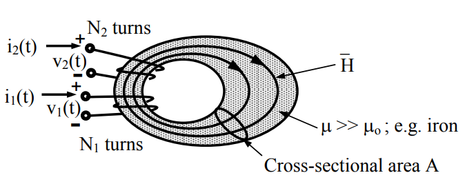
Its high permeability traps the magnetic flux within it so that \( \psi_{\text{m}}\) is constant around the toroid, even though A varies. From (3.2.28) we see that the voltage v_k across coil k is therefore:

\[\text{v}_{\text{k}}=\text{d} \Lambda_{\text{k}} / \text{d} \text{t}=\text{N}_{\text{k}} \text{d} \Psi_{\text{m}} / \text{d} \text{t}\]

The ratio between the voltages across two coils k = 1,2 is therefore:

\[\text{v}_{2} / \text{v}_{1}=\text{N}_{2} / \text{N}_{1} \]

where N₂/N₁ is the transformer turns ratio.

If current i₂ flows in the output coil, then there will be an added contribution to v₁ and v₂ due to the contributions of i₂ to the original \(\psi_{\text{m}}\) from the input coil alone. Note that current flowing into the “+” terminal of both coils in the figure contribute to \(\overline H\) in the illustrated direction; this distinguishes the positive terminal from the negative terminal of each coil. If the flux coupling between the two coils is imperfect, then the output voltage is correspondingly reduced. Any resistance in the wires can increment these voltages in proportion to the currents.

Figure 3.2.8 suggests traditional symbols used to represent ideal transformers and some common configurations used in practice. The polarity dot at the end of each coil indicates which terminals would register the same voltage for a given change in the linked magnetic flux. In the absence of dots, the polarity indicated in (a) is understood. Note that many transformers consist of a single coil with multiple taps. Sometimes one of the taps is a commutator that can slide across the coil windings to provide a continuously variable transformer turns ratio. As illustrated, the presence of an iron core is indicated by parallel lines and an auto-transformer consists of only one tapped coil.

Figure \(\PageIndex{8}\): Transformer configurations:

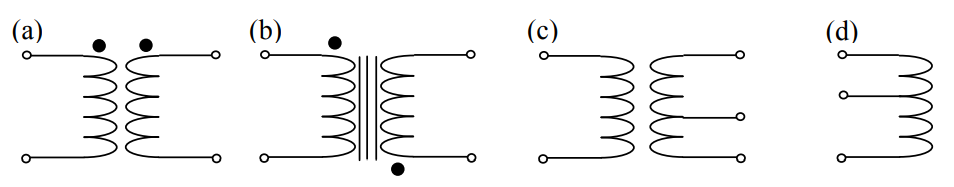
(a) air-core, (b) iron-core, (c) tapped, and (d) auto-transformer.

The terminal voltages of linear transformers for which μ ≠ f(H) are linearly related to the various currents flowing through the windings. Consider a simple toroid for which H, B, and the cross-sectional area A are the same everywhere around the average circumference \(\pi\)D. In this case the voltage \(\underline{V}_{1}\) across the N₁ turns of coil (1) is:

\[ \underline{V}_{1}=j \omega N_{1}\]

\[ \underline{\Psi}=\mu \underline{H}\text{A}\]

\[\underline{\text{H}}=\left(\text{N}_{1} \underline{\text{I}}_{1}+\text{N}_{2} \underline{\text{I}}_{2}\right) / \pi \text{D} \]

Therefore:

\[\underline{\text{V}}_{1}=\text{j} \omega\left[\mu \text{A} \text{N}_{1}\left(\text{N}_{1} {\underline{I}}_{1}+\text{N}_{2} {\underline{I}}_{2}\right) / \pi \text{D}\right]=\text{j} \omega\left(\text{L}_{11} \underline{\text{I}}_{1}+\text{L}_{12} {\underline{I}}_{2}\right) \]

where the self-inductance L₁₁ and mutual inductance L₁₂ [Henries] are:

\[\text{L}_{11}=\mu \text{AN}_{1}^{2} / \pi \text{D} \qquad\qquad \text{L}_{12}=\mu \text{AN}_{1} \text{N}_{2} / \pi \text{D}\]

Equation (3.2.35) can be generalized for a two-coil transformer:

\[\left[\frac{\mathrm{\underline{V}}_{1}}{\mathrm{\underline{V}}_{2}}\right]=\left[\begin{array}{ll} \mathrm{L}_{11} & \mathrm{L}_{12} \\ \mathrm{L}_{21} & \mathrm{L}_{22} \end{array}\right]\left[\frac{\underline{\mathrm{I}}_{1}}{\mathrm{\underline{I}}_{2}}\right] \]

Consider the simple toroidal step-up transformer illustrated in Figure 3.2.9 in which the voltage source drives the load resistor R through the transformer, which has N₁ and N₂ turns on its input and output, respectively. The toroid has major diameter D and cross-sectional area A.

Figure \(\PageIndex{9}\): Toroidal step-up transformer loaded with resistor R.

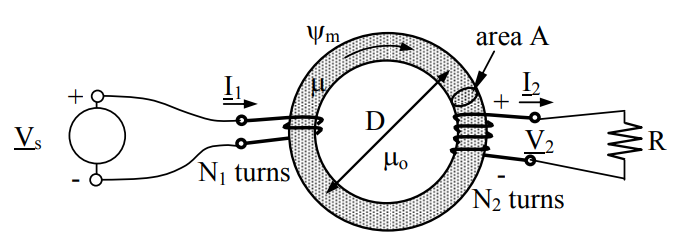
Combining (3.2.33) and (3.2.34), and noting that the sign of I₂ has been reversed in the figure, we obtain the expression for total flux:

\[\underline{\Psi}=\mu \text{A}\left(\text{N}_{1} \text{I}_{1}+\text{N}_{2} \underline{\text{I}}_{2}\right) / \pi \text{D}\]

We can find the admittance seen by the voltage source by solving (3.2.38) for \(\underline{I}_{1} \) and dividing by \(\underline{V}_{s} \):

\[ \underline{I}_{1}=\left(\pi D \underline{\Psi} / \mu \text{A} \text{N}_{1}\right)+\underline{\text{I}}_{2} \text{N}_{2} / \text{N}_{1}\]

\[\underline{\text{V}}_{\text{s}}=\text{j} \omega \text{N}_{1} \ \underline{\Psi}=\underline{\text{V}}_{2} \text{N}_{1} / \text{N}_{2}=\underline{\text{I}}_{2} \text{R} \text{N}_{1} / \text{N}_{2} \]

\[\begin{align} \underline{I}_{1} / \underline{V}_{s} &=\left(\pi D \underline{\Psi} / \mu \text{A} \text{N}_{1}\right) / \text{j} \omega \text{N}_{1} \underline{\Psi}+\underline{\text{I}}_{2} \text{N}_{2}^{2} /\left(\text{N}_{1}^{2} \underline{\text{I}}_{2} \text{R}\right) \\ &=-\text{j} \pi \text{D} /\left(\omega \text{N}_{1}^{2} \mu \text{A}\right)+\left(\text{N}_{2} / \text{N}_{1}\right)^{2} / \text{R}=1 / \text{j} \omega \text{L}_{11}+\left(\text{N}_{2} / \text{N}_{1}\right)^{2} / \text{R} \end{align} \]

Thus the admittance seen at the input to the transformer is that of the self-inductance (1/jωL₁₁) in parallel with the admittance of the transformed resistance [(N₂/N₁)²/R]. The power delivered to the load is \(\left|\underline{\text{V}}_{2}\right|^{2} / 2 \text{R}=\left|{\underline{V}}_{1}\right|^{2}\left(\text{N}_{2} / \text{N}_{1}\right)^{2} / 2 \text{R} \), which is the time-average power delivered to the transformer, since \( \left|{\underline{V}}_{2}\right|^{2}=\left|\underline{\text{V}}_{1}\right|^{2}\left(\text{N}_{2} / \text{N}_{1}\right)^{2}\); see (3.2.31).

The transformer equivalent circuit is thus L₁₁ in parallel with the input of an ideal transformer with turns ratio N₂/N₁. Resistive losses in the input and output coils could be represented by resistors in series with the input and output lines. Usually jωL₁₁ for an iron-core transformer is so great that only the ideal transformer is important.

One significant problem with iron-core transformers is that the changing magnetic fields within them can generate considerable voltages and eddy currents by virtue of Ohm’s Law ( \( \underline{\overline{\mathrm{J}}} \) = σ \( \overline{\underline{E}}\) ) and Faraday’s law:

\[\oint_{\text{C}} \underline{\overline{E}} \bullet \text{d} \overline{\text{s}}=-\text{j} \omega \mu \int_{\text{A}} \underline{\overline{H}} \bullet \text{d} \overline{\text{a}}\]

where the contour C circles each conducting magnetic element. A simple standard method for reducing the eddy currents \( \underline{\overline J}\) and the associated dissipated power \(\int_{V}\left(\sigma|\underline{J}|^{2} / 2\right) \text{d} \text{v}\) is to reduce the area A by laminating the core; i.e., by fabricating it with thin stacked insulated slabs of iron or steel oriented so as to interrupt the eddy currents. The eddy currents flow perpendicular to \(\overline{\text{H}}\), so the slab should be sliced along the direction of \(\overline{\text{H}}\). If N stacked slabs replace a single slab, then A, \( \underline{\text{E}}\), \(\underline{\text{J}} \) are each reduced roughly by a factor of N, so the power dissipated, which is proportional to the square of J, is reduced by a factor of ~N² . Eddy currents and laminated cores are discussed further at the end of Section 4.3.3.