3.3: Quasistatic Behavior of Devices

Electroquasistatic Behavior of Devices

The voltages and currents associated with all interesting devices sometimes vary. If the wavelength λ = c/f associated with these variations is much larger than the device size D, no significant wave behavior can occur. The device behavior can then be characterized as electroquasistatic if the device stores primarily electric energy, and magnetoquasistatic if the device stores primarily magnetic energy. Electroquasistatics involves the behavior of electric fields plus the first-order magnetic consequences of their variations. The electroquasistatic approximation includes the magnetic field⎯H generated by the varying dominant electric field (Ampere’s law), where:

\[\nabla \times \overline{\mathrm{H}}=\sigma \overline{\mathrm{E}}+\frac{\partial \overline{\mathrm{D}}}{\partial \mathrm{t}}\]

The quasistatic approximation neglects the second-order electric field contributions from the time derivative of the resulting \(\overline H\) in Faraday’s law:

\[\nabla \times \overline{\mathrm{E}}=-\mu_{\mathrm{o}} \partial \overline{\mathrm{H}} / \partial \mathrm{t} \cong 0. \nonumber\]

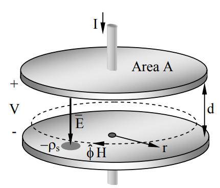
One simple geometry involving slowly varying electric fields is a capacitor charged to voltage V(t), as illustrated in Figure 3.3.1. It consists of two circular parallel conducting plates of diameter D and area A that are separated in vacuum by the distance d << D. Boundary conditions require \(\overline E\) to be perpendicular to the plates, where E(t) = V(t)/d, and the surface charge density is given by (2.6.15):

\[\overline{\mathrm{E}} \bullet \hat{\mathrm{n}}=\rho_{\mathrm{s}} / \varepsilon_{\mathrm{o}}=\mathrm{V} / \mathrm{d}\]

\[\rho_{\mathrm{s}}=\varepsilon_{\mathrm{o}} \mathrm{V} / \mathrm{d}\ \left[\mathrm{C} \mathrm{m}^{-2}\right]\]

Figure \(\PageIndex{1}\): Quasistatic electric and magnetic fields in a circular capacitor.

Since the voltage across the plates is the same everywhere, so are \( \overline E\) and ρ_s, and therefore the total charge is:

\[\mathrm{Q}(\mathrm{t}) \cong \rho_{\mathrm{s}} \mathrm{A} \cong\left(\varepsilon_{\mathrm{o}} \mathrm{A} / \mathrm{d}\right) \mathrm{V}=\mathrm{CV}(\mathrm{t})\]

where C ≅ ε_oA/d is the capacitance, as shown earlier (3.1.10). The same surface charge density ρ_s(t) can also be found by evaluating first the magnetic field \(\overline{\mathrm{H}}(\mathrm{r}, \mathrm{t})\) produced by the slowly varying (quasistatic) electric field \(\overline{\mathrm{E}}(\mathrm{t})\), and then the surface current \(\overline{\mathrm{J}}_{\mathrm{s}}(\mathrm{r}, \mathrm{t})\) associated with \(\overrightarrow{\mathrm{H}}(\mathrm{r}, \mathrm{t})\); charge conservation then links \(\overline{\mathrm{J}}_{\mathrm{s}}(\mathrm{r}, \mathrm{t})\) to ρ_s(t).

Ampere’s law requires a non-zero magnetic field between the plates where \(\overline J\) = 0:

\[\oint_{\mathrm{C}} \overline{\mathrm{H}} \bullet \mathrm{d} \overline{\mathrm{s}}=\varepsilon_{\mathrm{o}} \int \int_{\mathrm{A}^{\prime}}(\partial \overline{\mathrm{E}} / \partial \mathrm{t}) \cdot \mathrm{d} \overline{\mathrm{a}} \]

Symmetry of geometry and excitation requires that \(\overline H\) between the plates be in the \(\hat{\phi}\) direction and a function only of radius r, so (3.3.5) becomes:

\[2 \pi r H(r)=\varepsilon_{0} \pi r^{2} d E / d t=\left(\varepsilon_{0} \pi r^{2} / d\right) d V / d t \]

\[ \mathrm{H}(\mathrm{r})=\left(\varepsilon_{\mathrm{o}} \mathrm{r} / 2 \mathrm{d}\right) \mathrm{d} \mathrm{V} / \mathrm{d} \mathrm{t}\]

If V(t) and the magnetic field H are varying so slowly that the electric field given by Faraday’s law for H(r) is much less than the original electric field, then that incremental electric field can be neglected, which is the essence of the electroquasistatic approximation. If it cannot be neglected, then the resulting solution becomes more wavelike, as discussed in later sections.

The boundary condition \(\hat{\mathrm{n}} \times \overline{\mathrm{H}}=\overline{\mathrm{J}}_{\mathrm{s}} \) (2.6.17) then yields the associated surface current \(\overline{J}_{s}(r) \) flowing on the interior surface of the top plate:

\[ \overline{J}_{s}(r)=\hat{r}\left(\varepsilon_{0} r / 2 d\right) d V / d t=\hat{r} J_{s r}\]

This in turn is related to the surface charge density ρ_s by conservation of charge (2.1.19), where the del operator is in cylindrical coordinates:

\[ \nabla \bullet \overline{\mathrm{J}}_{\mathrm{s}}=-\partial \rho_{\mathrm{s}} / \partial \mathrm{t}=-\mathrm{r}^{-1} \partial\left(\mathrm{r} \mathrm{J}_{\mathrm{sr}}\right) / \partial \mathrm{r}\]

Substituting \(J_{sr}\) from (3.3.8) into the right-hand side of (3.3.9) yields:

\[\partial \rho_{\mathrm{s}} / \partial \mathrm{t}=\left(\varepsilon_{\mathrm{o}} / \mathrm{d}\right) \mathrm{d} \mathrm{V} / \mathrm{d} \mathrm{t}\]

Multiplying both sides of (3.3.10) by the plate area A and integrating over time then yields Q(t) = CV(t), which is the same as (3.3.4). Thus we could conclude that variations in V(t) will produce magnetic fields between capacitor plates by virtue of Ampere’s law and the values of either \(\partial \overline{\mathrm{D}} / \partial \mathrm{t} \) between the capacitor plates or \( \overline{\mathrm{J}}_{\mathrm{s}}\) within the plates. These two approaches to finding \(\overline H\) (using \(\partial \overline{\mathrm{D}} / \partial \mathrm{t}\) or \(\overline{J}_{s}\)) yield the same result because of the self-consistency of Maxwell’s equations.

Because the curl of \(\overline H\) in Ampere’s law equals the sum of current density \(\overline J\) and \(\partial \overline{\mathrm{D}} / \partial \mathrm{t}\), the derivative \(\partial \overline{\mathrm{D}} / \partial \mathrm{t}\) is often called the displacement current density because the units are the same, A/m² . For the capacitor of Figure 3.3.1 the curl of \(\overline H\) near the feed wires is associated only with \(\overline J\) (or I), whereas between the capacitor plates the curl of \(\overline H\) is associated only with displacement current.

Section 3.3.4 treats the electroquasistatic behavior of electric fields within conductors and relaxation phenomena.

Magnetoquasistatic behavior of devices

All currents produce magnetic fields that in turn generate electric fields if those magnetic fields vary. Magnetoquasistatics characterizes the behavior of such slowly varying fields while neglecting the second-order magnetic fields generated by \(\partial \overline{\mathrm{D}} / \partial \mathrm{t}\) in Ampere’s law, (2.1.6):

\[ \nabla \times \overline{\mathrm{H}}=\overline{\mathrm{J}}+\partial \overline{\mathrm{D}} / \partial \mathrm{t} \cong \overline{\mathrm{J}} \qquad\qquad\qquad \text { (quasistatic Ampere's law) }\]

The associated electric field \(\overline E\) can then be found from Faraday's law:

\[ \nabla \times \overline{\mathrm{E}}=-\partial \overline{\mathrm{B}} / \partial \mathrm{t} \qquad\qquad\qquad \text{(Faraday’s law)}\]

Section 3.2.1 treated an example for which the dominant effect of the quasistatic magnetic field in a current loop is voltage induced via Faraday’s law, while the example of a short wire follows; both are inductors. Section 3.3.4 treats the magnetoquasistatic example of magnetic diffusion, which is dominated by currents induced by the first-order induced voltages, and resulting modification of the original magnetic field by those induced currents. In every quasistatic problem wave effects can be neglected because the associated wavelength λ >> D, where D is the maximum device dimension.

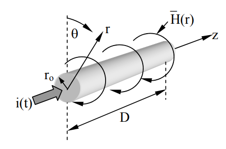
We can roughly estimate the inductance of a short wire segment by modeling it as a perfectly conducting cylinder of radius r_o and length D carrying a current i(t), as illustrated in Figure 3.3.2. An exact computation would normally be done using computer tools designed for such tasks because analytic solutions are practical only for extremely simple geometries. In this analysis we neglect any contributions to \(\overline H\) from currents in nearby conductors, which requires those nearby conductors to have much larger diameters or be far away. We also make the quasistatic assumption λ >> D.

Figure \(\PageIndex{2}\): Inductance of an isolated wire segment.

We know from (3.2.23) that the inductance of any device can be expressed in terms of the magnetic energy stored as a function of its current i:

\[\mathrm{L}=2 \mathrm{w}_{\mathrm{m}} / \mathrm{i}^{2} \ [\mathrm{H}]\]

Therefore to estimate L we first estimate \(\overline H \) and w_m. If the cylinder were infinitely long then \(\overline{\mathrm{H}} \cong \hat{\theta} \mathrm{H}(\mathrm{r})\) must obey Ampere’s law and exhibit the same cylindrical symmetry, as suggested in the figure. Therefore:

\[\oint_{C} \overline{H} \bullet d \overline{s}=2 \pi r H(r)=i(t)\]

and H(r) ≅ i/2\(\pi\)r . Therefore the instantaneous magnetic energy density is:

\[\left\langle\mathrm{W}_{\mathrm{m}}\right\rangle=\frac{1}{2} \mu_{\mathrm{o}} \mathrm{H}^{2}(\mathrm{r})=\frac{1}{2} \mu_{\mathrm{o}}(\mathrm{i} / 2 \pi \mathrm{r})^{2} \ \left[\mathrm{J} / \mathrm{m}^{3}\right]\]

To find the total average stored magnetic energy we must integrate over volume. Laterally we can neglect fringing fields and simply integrate over the length D. Integration with respect to radius will produce a logarithmic answer that becomes infinite if the maximum radius is infinite. A plausible outer limit for r is ~D because the Biot-Savart law (1.4.6) says fields decrease as r² from their source if that source is local; the transition from slow cylindrical field decay as r^-1 to decay as r^-2 occurs at distances r comparable to the largest dimension of the source: r ≅ D. With these approximations we find:

\[\begin{aligned} \mathrm{w}_{\mathrm{m}} & \cong \int_{0}^{\mathrm{D}} \mathrm{d} \mathrm{z} \int_{\mathrm{r}_{0}}^{\mathrm{D}}\left\langle\mathrm{W}_{\mathrm{m}}\right\rangle 2 \pi \mathrm{r} \mathrm{dr} \cong \mathrm{D} \int_{\mathrm{r}_{0}}^{\mathrm{D}} \frac{1}{2} \mu_{\mathrm{o}}\left(\frac{\mathrm{i}}{2 \pi \mathrm{r}}\right)^{2} 2 \pi \mathrm{r} \mathrm{dr} \\ &=\left.\left(\mu_{\mathrm{o}} \mathrm{Di}^{2} / 4 \pi\right) \ln \mathrm{r}\right|_{\mathrm{ro}} ^{\mathrm{D}}=\left(\mu_{\mathrm{o}} \mathrm{Di}^{2} / 4 \pi\right) \ln \left(\mathrm{D} / \mathrm{r}_{\mathrm{o}}\right) \ [\mathrm{J}] \end{aligned}\]

Using (3.3.13) we find the inductance L for this wire segment is:

\[\mathrm{L} \cong\left(\mu_{\mathrm{o}} \mathrm{D} / 2 \pi\right) \ln \left(\mathrm{D} / \mathrm{r}_{\mathrm{o}}\right) \ [\mathrm{Hy}]\]

where the units “Henries” are abbreviated here as “Hy”. Note that superposition does not apply here because we are integrating energy densities, which are squares of field strengths, and the outer limit of the integral (3.3.16) is wire length D, so longer wires have slightly more inductance than the sum of shorter elements into which they might be subdivided.

Equivalent circuits for simple devices

Section 3.1 showed how the parallel plate resistor of Figure 3.1.1 would exhibit resistance R = d/σA ohms and capacitance C = εA/d farads, connected in parallel. The currents in the same device also generate magnetic fields and add inductance.

Referring to Figure 3.1.1 of the original parallel plate resistor, most of the inductance will arise from the wires, since they have a very small radius r_o compared to that of the plates. This inductance L will be in series with the RC portions of the device because their two voltage drops add. The R and C components are in parallel because the total current through the device is the sum of the conduction current and the displacement current, and the voltages driving these two currents are the same, i.e., the voltage between the parallel plates. The corresponding first-order equivalent circuit is illustrated in Figure 3.3.3.

Figure \(\PageIndex{3}\): Equivalent RLC circuit of a parallel-plate capacitor.

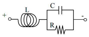
Examination of Figure 3.3.3 suggests that at very low frequencies the resistance R dominates because, relative to the resistor, the inductor and capacitor become approximate short and open circuits, respectively. At the highest frequencies the inductor dominates. As f increases from zero beyond where R dominates, either the RL or the RC circuit first dominates, depending on whether C shorts the resistance R at lower frequencies than when L open-circuits R; that is, RC dominates first when \(\mathrm{R}>\sqrt{\mathrm{L} / \mathrm{C}}\). At still higher frequencies the LC circuit dominates, followed by L alone. For certain combinations of R, L, and C, some transitions can merge.

Even this model for a resistor is too simple; for example, the wires also exhibit resistance and there is magnetic energy stored between the end plates because ∂D dt ≠ 0 there. Since such parasitic effects typically become important only at frequencies above the frequency range specified for the device, they are normally neglected. Even more complex behavior can result if the frequencies are so high that the device dimensions exceed ~λ/8, as discussed later in Section 7.1. Similar considerations apply to every resistor, capacitor, inductor, or transformer manufactured. Components and circuits designed for very high frequencies minimize unwanted parasitic capacitance and parasitic inductance by their very small size and proper choice of materials and geometry. It is common for circuit designers using components or wires near their design limits to model them with simple lumped-element equivalent circuits like that of Figure 3.3.3, which include the dominant parasitic effects. The form of these circuits obviously depends on the detailed structure of the modeled device; for example, R and C might be in series.

Example \(\PageIndex{A}\)

What are the approximate values L and C for the 100-Ω resistor designed in Example 3.1A if ε = 4ε_o, and what are the three critical frequencies (RC)^-1, R/L, and (LC)^-0.5?

Solution

The solution to 3.1A said the conducting caps of the resistor have area A = \(\pi\)r² = \(\pi\)(2.5×10^-4)² , and the length of the dielectric d is 1 mm. The permittivity ε = 4ε_o, so the capacitance (3.1.10) is

\[\begin{align*} C &= \dfrac{εA}{d} \\[4pt] &= 4 \times 8.85 \times 10^{-12} \pi (2.5×10^{-4})^2 /10^{-3} \\[4pt] &≅ 7 \times 10^{-15} \, \text{farads}. \end{align*}\]

The inductance L of this device would probably be dominated by that of the connecting wires because their diameters would be smaller and their length longer. Assume the wire length is D = 4d = 4×10^-3, and its radius r is 10^-4. Then (3.3.17) yields

L ≅ (μ_oD/16\(\pi\))ln(D/r) = (1.26×10^-6 × 4×10^-3/16\(\pi\))ln(40) = 3.7×10^-10 [Hy].

The critical frequencies R/L, (RC)^-1, and (LC)^-0.5 are 2.7×10¹¹, 6.2×10¹¹, and 1.4×10¹² [r s^-1], respectively, so the maximum frequency for which reasonably pure resistance is obtained is ~10 GHz (~R/2\(\pi\)L4)