4.2: Mirror image charges and currents
- Page ID
- 25000

One very useful problem solving technique is to change the problem definition to one that is easier to solve but is known to have the same answer. An excellent example of this approach is the use of mirror-image charges and currents, which also works for wave problems.10
10 Another example of this approach is use of duality between \(\overline{\mathrm{E}}\) and \(\overline{\mathrm{H}}\), as discussed in Section 9.2.6.
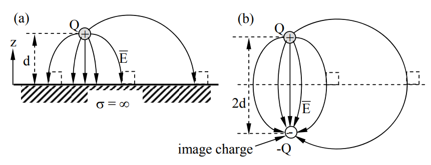
Consider the problem of finding the fields produced by a charge located a distance d above an infinite perfectly conducting plane, as illustrated in Figure 4.2.1(a). Boundary conditions at the conductor require only that the electric field lines be perpendicular to its surface. Any other set of boundary conditions that imposes the same constraint must yield the same unique solution by virtue of the uniqueness theorem of Section 2.8.
One such set of equivalent boundary conditions invokes a duplicate mirror image charge a distance 2d away from the original charge and of opposite sign; the conductor is removed. The symmetry for equal and opposite charges requires the electric field lines \(\overline{\mathrm{E}}\) to be perpendicular to the original surface of the conductor at z = 0; this results in \(\overline{\mathrm{E}}\) being exactly as it was for z > 0 when the conductor was present, as illustrated in Figure 4.2.1(b). Therefore uniqueness says that above the half-plane the fields produced by the original charge plus its mirror image are identical to those of the original problem. The fields below the original half plane are clearly different, but they are not relevant to the original problem.
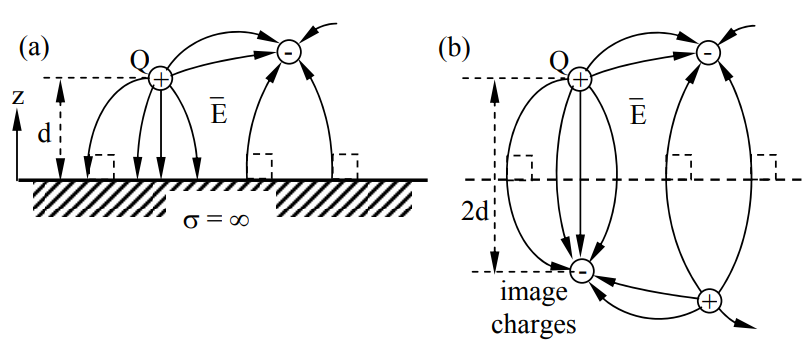
This equivalence applies for multiple charges or for a charge distribution, as illustrated in Figure 4.2.2. In fact the mirror image method remains valid so long as the charges change value or position slowly with respect to the relaxation time ε/σ of the conductor, as discussed in Section 4.4.1. The relaxation time is the 1/e time constant required for the charges within the conductor to approach new equilibrium positions after the source charge distribution outside changes.
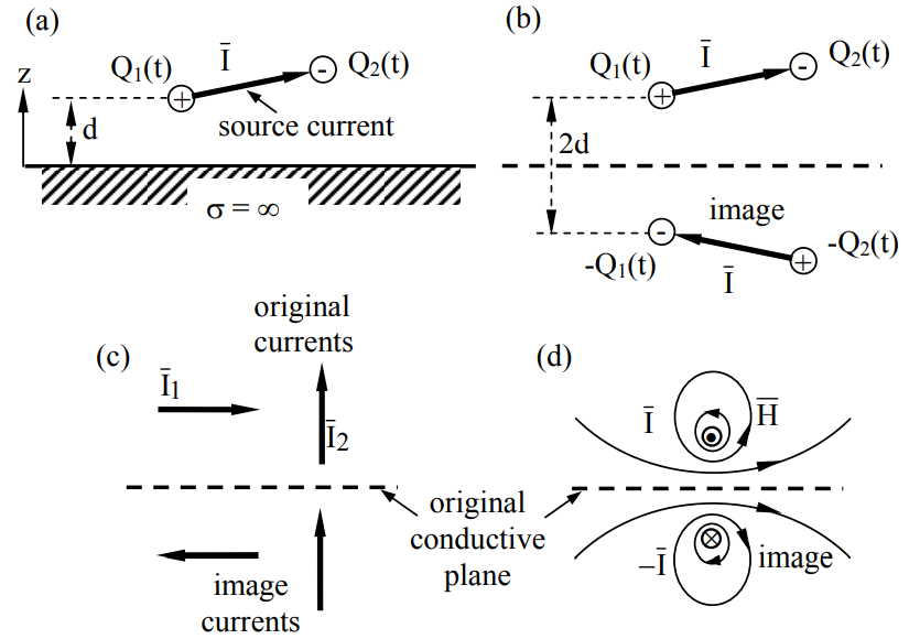
Because the mirror image method works for varying or moving charges, it works for the currents that must be associated with them by conservation of charge (2.1.21), as suggested in Figure 4.2.3 (a) and (b). Figure 4.2.3(d) also suggests how the magnetic fields produced by these currents satisfy the boundary conditions for the conducting plane: at the surface of a perfect conductor \(\overline{\mathrm{H}}\) is only parallel.
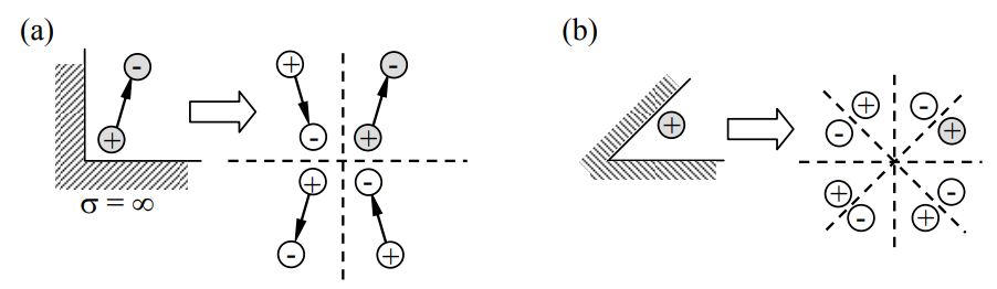
The mirror image method continues to work if the upper half plane contains a conductor, as illustrated in Figure 4.2.4; the conductor must be imaged too. These conductors can even be at angles, as suggested in Figure 4.2.4(b). The region over which the deduced fields are valid is naturally restricted to the original opening between the conductors. Still more complex image configurations can be used for other conductor placements, and may even involve an infinite series of progressively smaller image charges and currents.