5.2: Forces on Charges and Currents within Conductors

Electric Lorentz forces on charges within conductors

Static electric forces on charges within conductors can also be calculated using the Lorentz force equation (5.1.1), which becomes \(\overline{\mathrm{f}}=\mathrm{q} \overline{\mathrm{E}} \). For example, consider the capacitor plates illustrated in Figure 5.2.1(a), which have total surface charges of ±Q coulombs on the two conductor surfaces facing each other. The fields and charges for capacitor plates were discussed in Section 3.1.3.

Figure \(\PageIndex{1}\): Charge distribution within conducting capacitor plates.

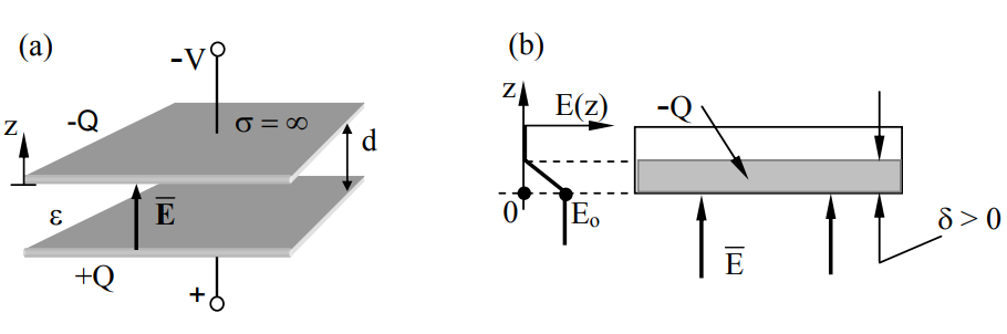
To compute the total attractive electric pressure P_e [N m^-2] on the top plate, for example, we can on the top plate, for example, we can integrate the Lorentz force density \(\overline{\mathrm{F}}\) [N m^-3] acting on the charge distribution ρ(z) over depth z and unit area:

\[\overline{\mathrm{F}}=\rho \overline{\mathrm{E}} \quad\left[\mathrm{N} \mathrm{m}^{-3}\right] \]

\[ \overline{\mathrm{P}}_{\mathrm{e}}=\int_{0}^{\infty} \overline{\mathrm{F}}(\mathrm{z}) \mathrm{d} \mathrm{z}=\hat{z} \int_{0}^{\infty} \rho(\mathrm{z}) \mathrm{E}_{\mathrm{z}}(\mathrm{z}) \mathrm{d} \mathrm{z} \quad\left[\mathrm{N} \mathrm{m}^{-2}\right]\]

where we have defined \( \overline{\mathrm{E}}=\hat{z} \mathrm{E}_{\mathrm{z}}\), as illustrated.

Care is warranted, however, because surface the charge ρ(z) is distributed over some infinitesimal depth δ, as illustrated in Figure 5.2.1(b), and those charges at greater depths are shielded by the others and therefore see a smaller electric field \( \overline{\mathrm{E}}\). If we assume ε = ε_o inside the conductors and a planar geometry with ∂/∂x = ∂/∂y = 0, then Gauss’s law, \(\nabla \bullet \varepsilon \overline{\mathrm{E}}=\rho \), becomes:

\[\varepsilon_{\mathrm{o}} \mathrm{d} \mathrm{E}_{\mathrm{z}} / \mathrm{d} \mathrm{z}=\rho(\mathrm{z})\]

This expression for ρ(z) can be substituted into (5.2.2) to yield the pressure exerted by the electric fields on the capacitor plate and perpendicular to it:

\[P_{e}=\int_{E_{0}}^{0} \varepsilon_{0} d E_{z} E_{z}=-\varepsilon_{0} E_{o}^{2} / 2 \qquad\qquad\qquad \text{(electric pressure on conductors) }\]

The charge density ρ and electric field E_z are zero at levels below δ, and the field strength at the surface is E_o. If the conductor were a dielectric with ε ≠ ε_o, then the Kelvin polarization forces discussed in Section 5.3.2 would also have to be considered.

Thus the electric pressure P_e [N m^-2] pulling on a charged conductor is the same as the immediately adjacent electric energy density [Jm^-3], and is independent of the sign of ρ and \(\overline{\mathrm{E}}\). These dimensions are identical because [J] = [Nm]. The maximum achievable electric field strength thus limits the maximum achievable electric pressure P_e, which is negative because it pulls rather than pushes conductors.

An alternate form for the electric pressure expression is:

\[P_{e}=-\varepsilon_{0} E_{0}^{2} / 2=-\rho_{s}^{2} / 2 \varepsilon_{0} \quad\left[\mathrm{Nm}^{-2}\right] \qquad\qquad\qquad \text {(electric pressure on conductors) }\]

where ρ_s is the surface charge density [cm^-2] on the conductor and εo is its permittivity; boundary conditions at the conductor require D = ε_oE = σs. Therefore if the conductor were adjacent to a dielectric slab with ε ≠ ε_o, the electrical pressure on the conductor would still be determined by the surface charge, electric field, and permittivity ε_o within the conductor; the pressure does not otherwise depend on ε of adjacent rigid materials.

We can infer from (5.2.4) the intuitively useful result that the average electric field pulling on the charge Q is E/2 since the total pulling force f = - P_eA, where A is the area of the plate:

\[\mathrm{f}=-\mathrm{P}_{\mathrm{e}} \mathrm{A}=\mathrm{A} \varepsilon_{\mathrm{o}} \mathrm{E}^{2} / 2=\mathrm{AD}(\mathrm{E} / 2)=\mathrm{Q}(\mathrm{E} / 2)\]

If the two plates were both charged the same instead of oppositely, the surface charges would repel each other and move to the outer surfaces of the two plates, away from each other. Since there would now be no E between the plates, it could apply no force. However, the charges Q on the outside are associated with the same electric field strength as before, E = Q/ε_oA. These electric fields outside the plates therefore pull them apart with the same force density as before, P_e = - ε_oE² /2, and the force between the two plates is now repulsive instead of attractive. In both the attractive and repulsive cases we have assumed the plate width and length are sufficiently large compared to the plate separation that fringing fields can be neglected.

Example \(\PageIndex{A}\)

Some copy machines leave the paper electrically charged. What is the electric field E between two adjacent sheets of paper if they cling together electrically with a force density of 0.01 oz. ≅ 0.0025 N per square centimeter = 25 Nm^-2? If we slightly separate two such sheets of paper by 4 cm, what is the voltage V between them?

Solution

Electric pressure is P_e = -ε_oE² /2 [N m^-2], so E = (-2P_eε_o)^0.5 = (2×25/8.8×10^-12)^0.5 = 2.4 [MV/m]. At 4 cm distance this field yields ~95 kV potential difference between the sheets. The tiny charge involved renders this voltage harmless.

Magnetic Lorentz Forces on Currents in Conductors

The Lorentz force law can also be used to compute forces on electrons moving within conductors for which μ = μ_o. Computation of forces for the case μ ≠ μ_o is treated in Sections 5.3.3 and 5.4. If there is no net charge and no current flowing in a wire, the forces on the positive and negative charges all cancel because the charges comprising matter are bound together by strong inter- and intra-atomic forces.

Figure \(\PageIndex{2}\): Magnetic force on a current-carrying wire.

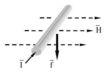
However, if n₁ carriers per meter of charge q are flowing in a wire¹⁵, as illustrated in Figure 5.2.2, then the total force density \(\overline{\mathrm{F}}=\mathrm{n}_{1} \mathrm{q} \overline{\mathrm{v}} \times \mu_{\mathrm{o}} \overline{\mathrm{H}}=\overline{\mathrm{I}} \times \mu_{\mathrm{o}} \overline{\mathrm{H}} \ \left[\mathrm{N} \mathrm{m}^{-1}\right]\) exerted by a static magnetic field \( \overline{\mathrm{H}}\) acting on the static current \(\overline{\mathrm{I}} \) flowing in the wire is:

\[\overline{\mathrm{F}}=\mathrm{n}_{1} \mathrm{q}^{-} \times \mu_{\mathrm{o}} \overline{\mathrm{H}}=\overline{\mathrm{I}} \times \mu_{\mathrm{o}} \overline{\mathrm{H}}\left[\mathrm{N} \mathrm{m}^{-1}\right] \qquad\qquad\qquad \text { (magnetic force density on a wire) }\]

where \( \overline{\mathrm{I}}=\mathrm{n}_{1} \mathrm{q} \overline{\mathrm{v}}\). If \(\overline{\mathrm{H}} \) is uniform, this force is not a function of the cross-section of the wire, which could be a flat plate, for example.

¹⁵ The notation n_j signifies number density [m^-j], so n₁ and n₃ indicate numbers per meter and per cubic meter, respectively.

Figure \(\PageIndex{3}\): Magnetic forces attracting parallel currents.

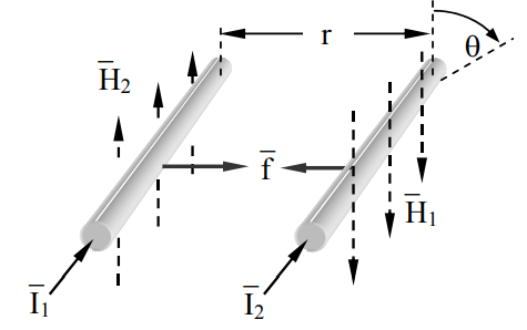
We can easily extend the result of (5.2.7) to the case of two parallel wires carrying the same current I in the same \(+\hat{z} \) direction and separated by distance r, as illustrated in Figure 5.2.3. Ampere’s law with cylindrical symmetry readily yields \(\overline{\mathrm{H}}(\mathrm{r})=\hat{\theta} \mathrm{H}(\mathrm{r}) \):

\[\oint_{\mathrm{c}} \overline{\mathrm{H}} \bullet \mathrm{d} \overline{\mathrm{s}}=\mathrm{I}=2 \pi \mathrm{rH} \Rightarrow \mathrm{H}=\mathrm{I} / 2 \pi \mathrm{r}\]

The force density \(\overline{\mathrm{F}} \) pulling the two parallel wires together is then found from (5.2.7) and (5.2.8) to be:

\[|\overline{\mathrm{F}}|=\mu_{\mathrm{o}} \mathrm{I}^{2} / 2 \pi \mathrm{r}\ \left[\mathrm{Nm}^{-1}\right]\]

The simplicity of this equation and the ease of measurement of F, I, and r led to its use in defining the permeability of free space, μ_o = 4\(\pi\)×10^-7 Henries/meter, and hence the definition of a Henry (the unit of inductance). If the two currents are in opposite directions, the force acting on the wires is repulsive. For example, if I = 10 amperes and r = 2 millimeters, then (5.2.9) yields F = 4\(\pi\)×10^-7 × 10² /2\(\pi\)²×10^-3 = 0.01 Newtons/meter; this is approximately the average repulsive force between the two wires in a 120-volt AC lamp cord delivering one kilowatt. These forces are attractive when the currents are parallel, so if we consider a single wire as consisting of parallel strands, they will squeeze together due to this pinch effect. At extreme currents, these forces can actually crush wires, so the maximum achievable instantaneous current density in wires is partly limited by their mechanical strength. The same effect can pinch electron beams flowing in charge-neutral plasmas.

The magnetic fields associated with surface currents on flat conductors generally exert a pressure \(\overline{\mathrm{P}} \ \left[\mathrm{N} \mathrm{m}^{-2}\right]\) that is simply related to the instantaneous field strength \(\left|\overline{\mathrm{H}}_{\mathrm{s}}\right| \) at the conductor surface. First we can use the magnetic term in the Lorentz force law (5.2.7) to compute the force density \(\overline{\mathrm{F}} \ \left[\mathrm{N} \mathrm{m}^{-3}\right] \) on the surface current \(\overline{\mathrm{J}}_{\mathrm{S}} \ \left[\mathrm{A} \mathrm{m}^{-1}\right] \):

\[\overline{\mathrm{F}}=\mathrm{nq} \overline{\mathrm{v}} \times \mu_{\mathrm{o}} \overline{\mathrm{H}}=\overline{\mathrm{J}} \times \mu_{\mathrm{o}} \overline{\mathrm{H}} \ \left[\mathrm{N} \mathrm{m}^{-3}\right]\]

where n is the number of charges q per cubic meter. To find the magnetic pressure P_m [N m^-2] on the conductor we must integrate the force density \(\overline{\mathrm{F}} \) over depth z, where both \( \overline{\mathrm{J}}\) and \( \overline{\mathrm{H}}\) are functions of z, as governed by Ampere’s law in the static limit:

\[\nabla \times \overline{\mathrm{H}}=\overline{\mathrm{J}}\]

If we assume \(\overline{\mathrm{H}}=\hat{y} \mathrm{H}_{\mathrm{y}} \ (\mathrm{z}) \) then \( \overline{\mathrm{J}}\) is in the x direction and ∂Hy/∂x = 0, so that:

\[\begin{align}
\nabla \times \overline{\mathrm{H}} &=\hat{x}\left(\partial \mathrm{H}_{\mathrm{z}} / \partial \mathrm{y}-\partial \mathrm{H}_{\mathrm{y}} / \partial \mathrm{z}\right)+\hat{y}\left(\partial \mathrm{H}_{\mathrm{x}} / \partial \mathrm{z}-\partial \mathrm{H}_{\mathrm{z}} / \partial \mathrm{x}\right)+\hat{z}\left(\partial \mathrm{H}_{\mathrm{y}} / \partial \mathrm{x}-\partial \mathrm{H}_{\mathrm{x}} / \partial \mathrm{y}\right) \\
&=-\hat{x} \mathrm{d} \mathrm{H}_{\mathrm{y}} / \mathrm{d} \mathrm{z}=\hat{x}_{\mathrm{x}}(\mathrm{z}) \nonumber
\end{align}\]

The instantaneous magnetic pressure P_m exerted by H can now be found by integrating the force density equation (5.2.10) over depth z to yield:

\[\overline{\mathrm{P}}_{\mathrm{m}}=\int_{0}^{\infty} \overline{\mathrm{F}} \mathrm{d} \mathrm{z}=\int_{0}^{\infty} \overline{\mathrm{J}}(\mathrm{z}) \times \mu_{\mathrm{o}} \overline{\mathrm{H}}(\mathrm{z}) \mathrm{d} \mathrm{z}=\int_{0}^{\infty}\left[-\hat{x} \mathrm{d} \mathrm{H}_{\mathrm{y}} / \mathrm{d} \mathrm{z}\right] \times\left[\hat{y} \mu_{\mathrm{o}} \mathrm{H}_{\mathrm{y}}(\mathrm{z})\right] \mathrm{d} \mathrm{z}\nonumber\]

\[\overline{\mathrm{P}}_{\mathrm{m}}=-\hat{z} \mu_{\mathrm{o}} \int_{\mathrm{H}}^{0} \mathrm{H}_{\mathrm{y}} \mathrm{d} \mathrm{H}_{\mathrm{y}}=\hat{z} \mu_{\mathrm{o}} \mathrm{H}^{2} / 2 \ \left[\mathrm{Nm}^{-2}\right] \qquad\qquad\qquad \text { (magnetic pressure) }\]

We have assumed \(\overline{\mathrm{H}}\) decays to zero somewhere inside the conductor. As in the case of the electrostatic pull of an electric field on a charged conductor, the average field strength experienced by the surface charges or currents is half that at the surface because the fields inside the conductor are partially shielded by any overlying charges or currents. The time average magnetic pressure for sinusoidal H is \(\left\langle\mathrm{P}_{\mathrm{m}}\right\rangle=\mu_{\mathrm{o}}|\overline{\mathrm{\underline{H}}}|^{2} / 4 \).