6.3: Rotary magnetic motors

Commutated rotary magnetic motors

Most electric motors and generators are rotary because their motion can then be continuous and high velocity, which improves power density and efficiency while prolonging equipment life. Figure 6.3.1 illustrates an idealized motor with a rotor comprising a single loop of wire carrying current I in the uniform magnetic field \(\overline{\mathrm{H}}\). The magnetic field can originate from permanent magnets in the stationary stator, which is the magnetic structure within which the rotor rotates, or from currents flowing in wires wrapped around the stator. The rotor typically has many turns of wire, often wrapped around a steel core with poles that nearly contact the stator along a cylindrical surface.

The total torque (force times radius) on the motor axle is found by adding the contributions from each of the four sides of the current loop; only the longitudinal elements of length W at radius \(\overline{\mathrm{r}}\) contribute, however. This total torque vector \(\overline{\mathrm{T}}=\overline{\mathrm{f}} \times \overline{\mathrm{r}}\) is the integral of the torque contributions from the force density F acting on each incremental length ds of the wire along its entire contour C:

\[\overline{\mathrm{T}}=\oint_{\mathrm{C}} \overline{\mathrm{r}} \times \overline{\mathrm{F}} \mathrm{d} \mathrm{s} \qquad\qquad\qquad\text{(torque on rotor)}\]

Figure \(\PageIndex{1}\): Rotary single-turn magnetic motor.

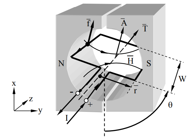
The force density \(\overline{\mathrm{F}} \) [N m^-1] on a wire conveying current \( \overline{\mathrm{I}}\) in a magnetic field \( \overline{\mathrm{H}}\) follows from the Lorentz force equation (5.1.1) and was given by (5.2.7):

\[ \overline{\mathrm{F}}=\overline{\mathrm{I}} \times \mu_{\mathrm{o}} \overline{\mathrm{H}} \ \left[\mathrm{N} \mathrm{m}^{-1}\right] \qquad \qquad \qquad \text { (force density on wire) }\]

Thus the torque for this motor at the pictured instant is clockwise and equals:

\[\overline{\mathrm{T}}=\hat{z} 2 \mathrm{rI} \mu_{\mathrm{o}} \mathrm{HW}\ [\mathrm{Nm}] \]

In the special case where \( \overline{\mathrm{H}}\) is uniform over the coil area A_o = 2rW, we can define the magnetic moment \(\overline{\mathrm{M}} \) of the coil, where \(|\overline{\mathrm{M}}|=\mathrm{IA}_{\mathrm{o}} \) and where the vector \(\overline{\mathrm{M}} \) is defined in a right hand sense relative to the current loop \(\overline{\mathrm{I}} \). Then:

\[\overline{\mathrm{T}}=\overline{\mathrm{M}} \times \mu_{\mathrm{o}} \overline{\mathrm{H}}\]

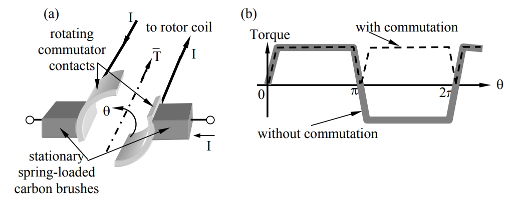
Because the current flows only in the given direction, \( \overline{\mathrm{H}}\) and the torque reverse as the wire loop passes through vertical (θ = n\(\pi\)) and have zero average value over a full rotation. To achieve positive average torque, a commutator can be added, which is a mechanical switch on the rotor that connects one or more rotor windings with one or more stationary current sources in the desired sequence and polarity. The commutator reverses the direction of current at times chosen so as to maximize the average positive torque. A typical configuration is suggested in Figure 6.3.2(a) where two spring-loaded carbon brushes pass the current I to the commutator contacts, which are rigidly attached to the rotor so as to reverse the current polarity twice per revolution. This yields the more nearly constant torque history T(θ) illustrated by the dashed line in Figure 6.3.2(b). In this approximate analysis of a DC motor we assume that the time constant L/R associated with the rotor inductance L and circuit resistance R is short compared to the torque reversals illustrated in Figure 6.3.2(b).

Figure \(\PageIndex{2}\): Commutator motor torque history and contact configuration.

Power is conserved, so if the windings are lossless then the average electrical power delivered to the motor, \(\mathrm{P}_{\mathrm{e}}=\langle\mathrm{VI}\rangle\), equals the average mechanical power delivered to the environment:

\[\mathrm{P}_{\mathrm{m}}=\mathrm{f}_{\mathrm{m}} \mathrm{v}_{\mathrm{m}}=\mathrm{f}_{\mathrm{m}} \mathrm{r}_{\mathrm{m}} \omega=\mathrm{T} \omega\]

where v_m is the velocity applied to the motor load by force f_m at radius r_m. If the motor is driven by a current source I, then the voltage across the rotor windings in this lossless case is:

\[\mathrm{V}=\mathrm{P}_{\mathrm{e}} / \mathrm{I}=\mathrm{P}_{\mathrm{m}} / \mathrm{I}=\mathrm{T} \omega / \mathrm{I}\]

This same voltage V across the rotor windings can also be deduced from the Lorentz force \( \overline{\mathrm{f}}=\mathrm{q}\left(\overline{\mathrm{E}}+\overline{\mathrm{v}} \times \mu_{\mathrm{o}} \overline{\mathrm{H}}\right)\), (6.1.1), acting on free conduction electrons within the wire windings as they move through \(\overline{\mathrm{H}}\). For example, if the motor is open circuit (I ≡ 0), these electrons spinning about the rotor axis at velocity \(\overline{\mathrm{v}}\) will move along the wire due to the "\( q \overline{\mathrm{v}} \times \mu_{\mathrm{o}} \overline{\mathrm{H}}\)" force on them until they have charged parts of that wire relative to other parts so as to produce a “\(q \overline{\mathrm{E}}\)” force that balances the local magnetic force, producing equilibrium and zero additional current. Free electrons in equilibrium have repositioned themselves so they experience no net Lorentz force. Therefore:

\[\overline{\mathrm{E}}=-\overline{\mathrm{v}} \times \mu_{\mathrm{o}} \overline{\mathrm{H}} \quad\left[\mathrm{V} \mathrm{m}^{-1}\right] \qquad \qquad\qquad\text { (electric field inside moving conductor) }\]

The integral of \(\overline{\mathrm{E}}\) from one end of the conducting wire to the other yields the open-circuit voltage \(\Phi\), which is the Thevenin voltage for this moving wire and often called the motor back voltage. \(\Phi\) varies only with rotor velocity and H, independent of any load. For the motor of Figure 6.3.1, Equation (6.3.7) yields the open-circuit voltage for a one-turn coil:

\[\Phi=2 \mathrm{EW}=2 \mathrm{v} \mu_{\mathrm{o}} \mathrm{HW}=2 \omega \mathrm{r} \mu_{\mathrm{o}} \mathrm{HW}=\omega \mathrm{A}_{\mathrm{o}} \mu_{\mathrm{o}} \mathrm{H} \ [\mathrm{V}] \qquad \qquad \qquad(\text { motor back-voltage })\]

where the single-turn coil area is A_o = 2rW. If the coil has N turns, then A_o is replaced by NA_o in (6.3.8).

The Thevenin equivalent circuits representing the motor and its external circuit determine the current I, as illustrated in Figure 6.3.3.

Figure \(\PageIndex{3}\): Equivalent circuit for a driven motor/generator.

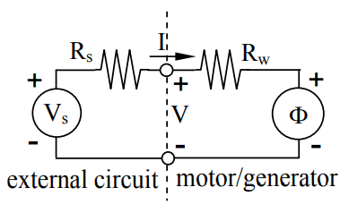
R_w is the winding resistance of the motor, where:

\[\mathrm{I}=\left(\mathrm{V}_{\mathrm{s}}-\Phi\right) /\left(\mathrm{R}_{\mathrm{s}}+\mathrm{R}_{\mathrm{w}}\right) \qquad \qquad \qquad \text { (motor current) }\]

When the motor is first starting, ω = \(\Phi\) = 0 and the current and the torque are maximum, where I_max = V_s/(R_s + R_w). The maximum torque, or “starting torque” from (6.3.3), where A_o = 2rW and there are N turns, is:

\[\overline{\mathrm{T}}_{\max }=\hat{\mathrm{z}} 2 \mathrm{WrNI}_{\max } \mu_{\mathrm{o}} \mathrm{H}=\hat{\mathrm{z}} \mathrm{NA}_{\mathrm{o}} \mathrm{I}_{\max } \mu_{\mathrm{o}} \mathrm{H}\ [\mathrm Nm]\]

Since \(\Phi\) = 0 when \(\overline{\mathrm{v}}=0\), , I\(\Phi\) = 0 and no power is converted then. As the motor accelerates toward its maximum ω, the back-voltage \(\Phi\) steadily increases until it equals the source voltage V_s so that the net driving voltage, torque T, and current I → 0 at ω = ω_max. Since (6.3.8) says \(\Phi\) = ωNA_oμ_oH, it follows that if \(\Phi\) = V_s, then:

\[\omega_{\max }=\frac{V_{s}}{N A_{o} \mu_{o} H}=\frac{V_{s} I_{\max }}{T_{\max }}\]

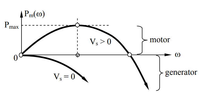
where the relation to T_max comes from (6.3.10), and ω_max occurs at T_min. = 0. At ω_max no power is being converted, so the maximum motor power output P_max occurs at an intermediate speed ω_p, as illustrated in Figure 6.3.4.

Figure \(\PageIndex{4}\): Mechanical power output P_m(ω) from a magnetic motor.

An expression for the mechanical output power P_m(ω) follows from (6.3.9):

\[P_{\mathrm{m}}=\mathrm{T} \omega=\mathrm{I} \Phi=\left(\mathrm{V}_{\mathrm{s}} \Phi-\Phi^{2}\right) /\left(\mathrm{R}_{\mathrm{s}}+\mathrm{R}_{\mathrm{w}}\right) \qquad \qquad \qquad \text{(mechanical power out)}\]

where (6.3.8) says \(\Phi\) = ωNA_oμ_oH, so P_m ∝ (V_sω - NA_oμ_oHω²).

Equation (6.3.12) says that if V_s >> \(\Phi\), which occurs for modest values of ω, then the motor power increases linearly with \(\Phi\) and ω. Also, if V_s = 0, then P_m is negative and the device acts as a generator and transfers electrical power to R_s + R_w proportional to \(\Phi^{2}\) and therefore ω². Moreover, if we differentiate P_m with respect to \(\Phi\) and set the result to zero, we find that the mechanical power is greatest when \(\Phi\) = V_s/2, which implies ω_p = ω_max/2. In either the motor or generator case, the maximum power transfer is usually limited by currents overheating the insulation or by high voltages causing breakdown. Even when no power is transferred, the backvoltage \(\Phi\) could cause breakdown if the device spins too fast. Semiconductor switches that may fail before the motor insulation are increasingly replacing commutators so the risk of excessive ω is often a design issue. In an optimum motor design, all failure types typically occur near the same loading levels or levels of likelihood.

Typical parameters for a commutated 2-inch motor of this type might be: 1) B = μoH = 0.4 Tesla (4000 gauss) provided by permanent magnets in the stator, 2) an N = 50-turn coil on the rotor with effective area A = 10^-3N [m²], 3) Vs = 24 volts, and 4) R_s + R_w = 0.1 ohm. Then it follows from (6.3.11), (6.3.12) for \(\Phi\) = V_s/2, and (6.3.10), respectively, that:

\[\omega_{\max }=V_{s} / \mu_{0} \mathrm{H A N}=24 /\left(0.4 \times 10^{-3} \times 50\right)=1200 \ \left[\mathrm{rs}^{-1}\right] \Rightarrow 11,460 \ [\mathrm{rpm}]^{25}\]

\[P_{\max }=\left(V_{s} \Phi-\Phi^{2}\right) /\left(R_{s}+R_{w}\right)=V_{s}^{2} /\left[4\left(R_{s}+R_{w}\right)\right] \ [W]=24^{2} / 0.4 \cong 1.4 \ [\mathrm{kW}]\]

\[\mathrm{T}_{\max }=\mathrm{AN} \mu_{\mathrm{o}} \mathrm{HI}_{\mathrm{max}}=\mathrm{A} \mu_{\mathrm{o}} \mathrm{HV}_{\mathrm{s}} /\left(\mathrm{R}_{\mathrm{s}}+\mathrm{R}_{\mathrm{w}}\right)=0.05 \times 0.4 \times 24 / 0.1=4.8 \ [\mathrm{Nm}]\]

²⁵ The abbreviation “rpm” means revolutions per minute.

In practice, most motors like that of Figure 6.3.1 wrap the rotor windings around a high permeability core with a thin gap between rotor and stator; this maximizes H near the current I. Also, if the unit is used as an AC generator, then there may be no need for the polarity-switching commutator if the desired output frequency is simply the frequency of rotor rotation.

Example \(\PageIndex{A}\)

Design a commutated DC magnetic motor that delivers maximum mechanical power of 1 kW at 600 rpm. Assume B = 0.2 Tesla and that the source voltage V_s = 50 volts.

Solution

Maximum mechanical power is delivered at ω_p = ω_max/2 (see Figure 6.3.4). Solving (6.3.13) yields NA_o = V_s/(ω_maxμ_oH) = = 50/(2×600×60×2\(\pi\)×0.2), = 5.53×10^-4, where ω_max corresponds to 1200 rpm. If N = 6, then the winding area 2rW = A_o ≅ 1 cm². To find I_max we use (6.3.14) to find the maximum allowed value of R_s + R_w = (V_s\(\Phi\) - \(\Phi^{2}\))/P_m. But when the delivered mechanical power P_mech is maximum, \(\Phi\) = Vs/2, so R_s + R_w = (50×25 - 25²)/10³ = 0.63Ω, which could limit N if the wire is too thin. I_max = V_s/(R_s + R_w) = = 50/0.63 = 80 [A]. The starting torque T_max = I_max(NA_o)μ_oH = = 80(5.53×10^-4)0.2 = 0.22 [N m]. This kilowatt motor occupies a fraction of a cubic inch and may therefore overheat because the rotor is small and its thermal connection with the external world is poor except through the axle. It is probably best used in short bursts between cooling-off periods. The I²R_w thermal power dissipated in the rotor depends on the wire design.

Reluctance motors

Reluctance motors combine the advantages of rotary motion with the absence of rotor currents and the associated rotary contacts. Figure 6.3.5 suggests a simple idealized configuration with only a single drive coil.

Figure \(\PageIndex{5}\): Two-pole single-winding reluctance motor.

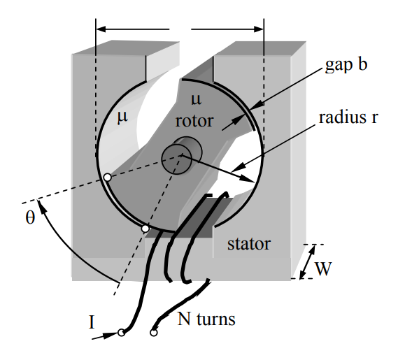
When the coil is energized the rotor is pulled by the magnetic fields into alignment with the magnetic fields linking the two poles of the stator, where μ >> μ_o in both the rotor and stator. Reluctance motors must sense the angular position of the rotor, however, so the stator winding(s) can be excited at the right times so as to pull the passive high-μ rotor toward its next rotary position, and then not retard it as it moves on toward the following attractive position. For example, the current I in the figure will pull the rotor so as to increase θ, which is the overlap angle between the rotor and the stator poles. Once the overlap is complete the current I would be set to zero as the rotor coasts until the poles again have θ ≅ 0 and are in position to be pulled forward again by I. Such motors are efficient if hysteresis losses in the stator and rotor are modest and the stator windings are nearly lossless.

The torque on such a reluctance motor can be readily calculated using (6.2.12):

\[\mathrm{T}=-\mathrm{d} \mathrm{w}_{\mathrm{T}} / \mathrm{d} \theta \ [\mathrm{Nm}]\]

The total magnetic energy w_T includes w_μ within the rotor and stator, w_g in the air gaps between them, and any energy in the power supply driving the motor. Fortunately we can simplify the problem by noting that w_g generally dominates, and that by short-circuiting the stator the same torque exists without any power source if I remains unchanged.

The circumstances for which the gap energy dominates the total energy w_T are easily found from the static integral form of Ampere’s law (1.4.1):

\[\mathrm{NI}=\oint_{\mathrm{C}}\left(\overline{\mathrm{H}}_{\mathrm{gap}}+\overline{\mathrm{H}}_{\mathrm{stator}}+\overline{\mathrm{H}}_{\mathrm{rotor}}\right) \bullet \mathrm{d} \overline{\mathrm{s}} \cong 2 \mathrm{b} \mathrm{H}_{\mathrm{gap}}\]

To derive an approximate result we may assume the coil has N turns, the width of each gap is b, and the contour C threads the coil and the rest of the motor over a distance ~2D, and through an approximately constant cross-section A; D is the rotor diameter. Since the boundary conditions in each gap require \(\overline{\mathrm{B}}_{\perp}\) be continuous, \(\mu \mathrm{H}_{\mu} \cong \mu_{\mathrm{o}} \mathrm{H}_{\mathrm{g}}\), where H_μ ≅ H_stator ≅ H_rotor and H_g ≡ H_gap. The relative energies stored in the two gaps and the rotor/stator are:

\[\mathrm{w}_{\mathrm{g}} \cong 2 \mathrm{bA}\left(\mu_{\mathrm{o}} \mathrm{H}_{\mathrm{g}}^{2} / 2\right)\]

\[\mathrm{w}_{\mathrm{r} / \mathrm{s}} \cong 2 \mathrm{DA}\left(\mu \mathrm{H}_{\mu}^{2} / 2\right)\]

Their ratio is:

\[\mathrm{w}_{\mathrm{g}} / \mathrm{w}_{\mathrm{r} / \mathrm{s}}=2 \mathrm{b}\left(\mu_{\mathrm{o}} / \mu\right)\left(\mathrm{H}_{\mathrm{g}} / \mathrm{H}_{\mu}\right)^{2} / 2 \mathrm{D}=\mathrm{b}\left(\mu / \mu_{\mathrm{o}}\right) / \mathrm{D}\]

Thus w_g >> w_μ if b/D >> μ_o/μ. Since gaps are commonly b ≅ 100 microns, and iron or steel is often used in reluctance motors, μ ≅ 3000, so gap energy w_g dominates if the motor diameter D << 0.3 meters. If this approximation doesn’t apply then the analysis becomes somewhat more complex because both energies must be considered; reluctance motors can be much larger than 0.3 meters and still function.

Under the approximations w_T ≅ w_g and A = gap area = rθW, we may compute the torque T using (6.3.16) and (6.3.18):²⁶

\[\mathrm{T}=-\mathrm{d} \mathrm{w}_{\mathrm{g}} / \mathrm{d} \theta=-\mathrm{b} \mu_{\mathrm{o}} \mathrm{d}\left(\mathrm{A}\left|\mathrm{H}_{\mathrm{g}}\right|^{2}\right) / \mathrm{d} \theta\]

²⁶ The approximate dependence (6.3.19) of w_r/s upon A = rθW breaks down when θ→0, since w_g doesn’t dominate then and (6.3.19) becomes approximate.

The θ dependence of H_g can be found from Faraday’s law by integrating \(\overline{\mathrm{E}}\) around the short circuited coil:

\[\oint_{\mathrm{c} \text { coil }} \overline{\mathrm{E}} \bullet \mathrm{d} \overline{\mathrm{s}}=-\mathrm{N} \oiint_{\mathrm{A}}(\mathrm{d} \overline{\mathrm{B}} / \mathrm{dt}) \bullet \mathrm{d} \overline{\mathrm{a}}=-\mathrm{d} \Lambda / \mathrm{d} \mathrm{t}=0\]

The flux linkage Λ is independent of θ and constant around the motor [contour C of (6.3.17)], so Λ, w_g and T are easily evaluated at the gap where the area is A = rθW:

\[\Lambda=\mathrm{N} \int_{\mathrm{A}} \overline{\mathrm{B}} \bullet \mathrm{d} \overline{\mathrm{a}}=\mathrm{NB}_{\mathrm{g}} \mathrm{A}=\mathrm{N} \mu_{\mathrm{o}} \mathrm{H}_{\mathrm{g}} \mathrm{r} \theta \mathrm{W}\]

\[\mathrm{w}_{\mathrm{g}}=2\left(\mu_{\mathrm{o}} \mathrm{H}_{\mathrm{g}}^{2} / 2\right) \mathrm{b} \mathrm{A}=\mathrm{b} \Lambda^{2} /\left(\mathrm{N}^{2} \mu_{\mathrm{o}} \mathrm{r} \theta \mathrm{W}\right)\]

\[\mathrm{T}=-\mathrm{d} \mathrm{w}_{\mathrm{g}} / \mathrm{d} \theta=\mathrm{b} \Lambda^{2} /\left(\mathrm{N}^{2} \mu_{\mathrm{o}} \mathrm{r} \mathrm{W} \theta^{2}\right)=\mathrm{r} 2\left(\mu_{\mathrm{o}} \mathrm{H}_{\mathrm{g}}^{2} / 2\right) \mathrm{Wb} \ [\mathrm{Nm}]\]

The resulting torque T in (6.3.25) can be interpreted as being the product of radius r and twice the force exerted at the leading edge of each gap (twice, because there are two gaps), where this force is the magnetic pressure μ_oH_g²/2 [N m^-2] times the gap area Wb projected on the direction of motion. Because the magnetic field lines are perpendicular to the direction of force, the magnetic pressure pushes rather than pulls, as it would if the magnetic field were parallel to the direction of force. Unfortunately, increasing the gap b does not increase the force, because it weakens H_g proportionately, and therefore weakens T ∝ H². In general, b is designed to be minimum and is typically limited to roughly 25-100 microns by thermal variations and bearing and manufacturing tolerances. The magnetic field in the gap is limited by the saturation field of the magnetic material, as discussed in Section 2.5.4.

The drive circuits initiate the current I in the reluctance motor of Figure 6.3.5 when the gap area rθW is minimum, and terminate it when that area becomes maximum. The rotor then coasts with I = 0 and zero torque until the area is again minimum, when the cycle repeats. Configurations that deliver continuous torque are more commonly used instead because of their smoother performance.

Figure \(\PageIndex{6}\): Reluctance motor with 3 stator and 4 rotor poles.

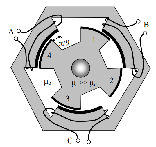
Figure 6.3.6 illustrates a reluctance motor that provides continuous torque using three stator poles (A, B, C) and four rotor poles (1, 2, 3, 4). When windings A and B are excited, rotor pole 1 is pulled clockwise into stator pole B. The gap area for stator pole A is temporarily constant and contributes no additional torque. After the rotor moves \(\pi\)/9 radians, the currents are switched to poles B and C so as to pull rotor pole 2 into stator pole C, while rotor pole 1 contributes no torque. Next C and A are excited, and this excitation cycle (A/B, B/C, C/A) is repeated six times per revolution. Counter-clockwise torque is obtained by reversing the excitation sequence. Many pole combinations are possible, and those with more poles yield higher torques because torque is proportional to the number of active poles. In this case only one pole is providing torque at once, so the constant torque \(\mathrm{T}=\mathrm{bW}\left(\mu_{0} \mathrm{H}_{\mathrm{g}}^{2} / 2\right)\) [N m].

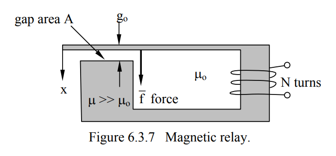
A calculation very similar to that above also applies to relays such as that illustrated in Figure 6.3.7, where a coil magnetizes a flexible or hinged bar, drawing it downward to open and/or close one or more electrical contacts.

Figure \(\PageIndex{7}\): Magnetic relay.

We can find the force f, flux linkage Λ, and gap energy w_g using a short-circuited N-turn coil to render Λ constant, as before:

\[\mathrm{f}=-\mathrm{d} \mathrm{w}_{\mathrm{g}} / \mathrm{d} \mathrm{x} \qquad\qquad\qquad \text{(force closing the gap)}\]

\[\Lambda=\mathrm{N} \mu_{\mathrm{o}} \mathrm{H}_{\mathrm{g}} \mathrm{A} \qquad\qquad\qquad \text{(flux linkage)}\]

\[\mathrm{w}_{\mathrm{g}}=\left(\mu_{\mathrm{o}} \mathrm{H}_{\mathrm{g}}^{2} / 2\right) \mathrm{A}\left(\mathrm{g}_{\mathrm{o}}-\mathrm{x}\right)=\left(\mathrm{g}_{\mathrm{o}}-\mathrm{x}\right) \Lambda^{2} /\left(2 \mathrm{N}^{2} \mu_{\mathrm{o}} \mathrm{A}\right)\ [\mathrm J] \qquad\qquad\qquad \text{(gap energy)}\]

\[\mathrm{f}=-\mathrm{d} \mathrm{w}_{\mathrm{g}} / \mathrm{d} \mathrm{x}=\Lambda^{2} /\left(2 \mathrm{N}^{2} \mu_{\mathrm{o}} \mathrm{A}\right)=\left(\mu_{\mathrm{o}} \mathrm{H}_{\mathrm{g}}^{2} / 2\right) \mathrm{A}\ [\mathrm{N}] \qquad\qquad\qquad \text{(force)}\]

This force can also be interpreted as the gap area A times a magnetic pressure P_m, where:

\[P_{m}=\mu_{0} H_{g}^{2} / 2 \ \left[\mathrm{N} / m^{2}\right] \qquad\qquad\qquad \text{(magnetic pressure)}\]

The magnetic pressure is attractive parallel to the field lines, tending to close the gap. The units N/m² are identical to J/m³. Note that the minus sign is used in (6.3.29) because f is the magnetic force closing the gap, which equals the mechanical force required to hold it apart; motion in the x direction reduces w_g.

Magnetic micro-rotary motors are difficult to build without using magnetic materials or induction²⁷ because it is difficult to provide reliable sliding electrical contacts to convey currents to the rotor. One form of rotary magnetic motor is similar to that of Figures 6.2.3 and 6.2.4, except that the motor pulls into the segmented gaps a rotating high-permeability material instead of a dielectric, where the gaps would have high magnetic fields induced by stator currents like those in Figure 6.3.6. As in the case of the rotary dielectric MEMS motors discussed in Section 6.2, the timing of the currents must be synchronized with the angular position of the rotor. The force on a magnetic slab moving into a region of strong magnetic field can be shown to approximate \(\mathrm{A} \mu \mathrm{H}_{\mu}^{2} / 2\) [N], where A is the area of the moving face parallel to H_μ, which is the field within the moving slab, and \(\mu>>\mu_{0}\). The rotor can also be made permanently magnetic so it is attracted or repelled by the synchronously switched stator fields; permanent magnet motors are discussed later in Section 6.5.2.

²⁷ Induction motors, not discussed in this text, are driven by the magnetic forces produced by a combination of rotor and stator currents, where the rotor currents are induced by the time-varying magnetic fields they experience, much like a transformer. This avoids the need for direct electrical contact with the rotor.

Example \(\PageIndex{B}\)

A relay like that of Figure 6.3.7 is driven by a current source I [A] and has a gap of width g. What is the force f(g) acting to close the gap? Assume the cross-sectional area A of the gap and metal is constant around the device, and note the force is depends on whether the gap is open or closed.

Solution

This force is the pressure \(\mu_{0} \mathrm{H}_{\mathrm{g}}^{2} / 2\) times the area A (6.3.29), assuming \(\mu>>\mu_{0}\). Since \(\nabla \times \overline{\mathrm{H}}=\overline{\mathrm{J}}\), therefore \(\mathrm{NI}=\oint \mathrm{H}(\mathrm{s}) \mathrm{ds}=\mathrm{H}_{\mathrm{g}} \mathrm{g}+\mathrm{H}_{\mu} \mathrm{S}\), where S is the path length around the loop having permeability μ. When \(\mathrm{H}_{\mathrm{g}} \mathrm{g}>>\mathrm{H}_{\mu} \mathrm{S}\), then \(\mathrm{H}_{\mathrm{g}} \cong \mathrm{NI} / \mathrm{g}\) and\(\mathrm{f} \cong \mu_{\mathrm{o}}(\mathrm{NI} / \mathrm{g})^{2} \mathrm{A} / 2\) for the open relay. When the relay is closed and g ≅0, then \(\mathrm{H}_{\mathrm{g}} \cong \mu \mathrm{H}_{\mathrm{u}} / \mu_{\mathrm{o}}\), where H_μ ≅ NI/S; then \(\mathrm{f} \cong(\mu \mathrm{NI} / \mathrm{S})^{2} \mathrm{A} / 2 \mu_{\mathrm{o}}\). The ratio of forces when the relay is closed to that when it is open is (μg/μ_oS)², provided \(\mathrm{H}_{\mathrm{g}} \mathrm{g}>>\mathrm{H}_{\mu} \mathrm{S}\) and this ratio \(>>1\).