7.4: TEM Resonances

Introduction

Resonators are widely used for manipulating signals and power, although unwanted resonances can sometimes limit system performance. For example, resonators can be used either as bandpass filters that remove all frequencies from a signal except those near the desired resonant frequency ω_n, or as band-stop filters that remove unwanted frequencies near ω_n and let all frequencies pass. They can also be used effectively as step-up transformers to increase voltages or currents to levels sufficient to couple all available energy into desired loads without reflections. That is, the matching circuits discussed in Section 7.3.2 can become sufficiently reactive for badly mismatched loads that they act like band-pass resonators that match the load only for a narrow band of frequencies. Although simple RLC resonators have but one natural resonance and complex RLC circuits have many, distributed electromagnetic systems can have an infinite number.

A resonator is any structure that can trap oscillatory electromagnetic energy so that it escapes slowly or not at all. Section 7.4.2 discusses energy trapped in TEM lines terminated so that outbound waves are reflected back into the resonator, and Section 9.4 treats cavity resonators formed by terminating rectangular waveguides with short circuits that similarly reflect and trap otherwise escaping waves. In each of these cases boundary conditions restricted the allowed wave structure inside to patterns having integral numbers of half- or quarter-wavelengths along any axis of propagation, and thus only certain discrete resonant frequencies ω_n can be present.

All resonators dissipate energy due to resistive losses, leakages, and radiation, as discussed in Section 7.4.3. The rate at which this occurs depends on where the peak currents or voltages in the resonator are located with respect to the resistive or radiating elements. For example, if the resistive element is in series at a current null or in parallel at a voltage null, there is no dissipation. Since dissipation is proportional to resonator energy content and to the squares of current or voltage, the decay of field strength and stored energy is generally exponential in time. Each resonant frequency f_n has its own rate of energy decay, characterized by the dimensionless quality factor \(Q_{n}\), which is generally the number of radians ω_nt required for the total energy w_Tn stored in mode n to decay by a factor of 1/e. More importantly, Q ≅ f_o/\(\delta\)f, where f_n is the resonant frequency and \(\delta\)f_n is the half-power full-width of resonance n.

Section 7.4.4 then discusses how resonators can be coupled to circuits for use as filters or transformers, and Section 7.4.5 discusses how arbitrary waveforms in resonators are simply a superposition of orthogonal modes, each decaying at its own rate.

TEM resonator frequencies

A resonator is any structure that traps electromagnetic radiation so it escapes slowly or not at all. Typical TEM resonators are terminated at their ends with lossless elements such as short- or open-circuits, inductors, or capacitors. Complex notation is used because resonators are strongly frequency-dependent. We begin with the expressions (7.1.55) and (7.1.58) for voltage and current on TEM lines:

\[\underline{V}(z)=\underline{V}_{+} \mathrm{e}^{-j \mathrm{k} z}+\underline{\mathrm{V}}_{-} \mathrm{e}^{+\mathrm{j} \mathrm{kz}}\ [\mathrm{V}]\]

\[\underline{I}(z)=Y_{o}\left[\underline{V}_{+} e^{-j k z}-\underline{V}_{-} e^{+j k z}\right] \ [A]\]

For example, if both ends of a TEM line of length D are open-circuited, then \(\underline{I}(z)=0\) at z = 0 and z = D. Evaluating (7.4.1) at z = 0 yields \(\underline{V}_{-}=\underline{V}_{+}\). At the other boundary:³⁶

\[\underline{I}(D)=0=Y_{0} \underline{V}_{+}\left(e^{-j k D}-e^{+j k D}\right)=-2 j Y_{0} \underline{V}_{+} \sin (k D)=-2 j Y_{0} \underline{V}_{+} \sin (2 \pi D / \lambda)\]

³⁶ We use the identity \(\sin \phi=\left(\mathrm{e}^{\mathrm{j} \phi}-\mathrm{e}^{-\mathrm{j} \phi}\right) / 2 \mathrm{j}\).

To satisfy (7.4.3), sin(2\(\pi\)D/λ) = 0, and so λ is restricted to specific resonances:

\[\lambda_{\mathrm{n}}=2 \mathrm{D} / \mathrm{n}=\mathrm{c} / \mathrm{f}_{\mathrm{n}} \text { for } \mathrm{n}=0,1,2,3, \ldots\]

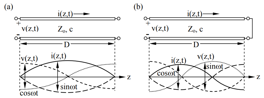
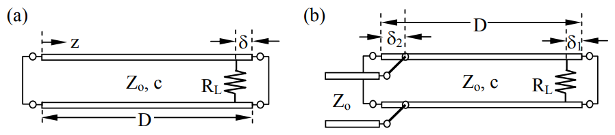
That is, at resonance the length of this open-circuited line is D = nλ_n/2, as suggested in Figure 7.4.1(a) for n = 1. The corresponding resonant frequencies are:

\[\mathrm f_{\mathrm n}=\mathrm c / \lambda_{\mathrm n}=\mathrm{n c} / 2 D \ \ [\mathrm{H z]}\]

By our definition, static storage of electric or magnetic energy corresponds to a resonance at zero frequency. For example, in this case the line can hold a static charge and store electric energy at zero frequency (n = 0) because it is open-circuited at both ends. Because the different modes of a resonator are spatially orthogonal, the total energy stored in a resonator is the sum of the energies stored in each of the resonances separately, as shown later in (7.4.20).

Figure \(\PageIndex{1}\): Voltage and current on TEM resonators.

The time behavior corresponding to (7.4.2) when \(2 \mathrm{Y}_{\mathrm{o}} \mathrm{\underline{V}}_{+}=\mathrm{I}_{\mathrm{o}}\) is:

\[i(t, z)=R_{e}\left\{\underline{I} e^{j \omega t}\right\}=I_{0} \sin \omega t \sin (2 \pi z / \lambda)\]

where ω = 2\(\pi\)c/λ. The corresponding voltage v(t,z) follows from (7.4.1), \(\underline{V}_{-}=\underline{V}_{+}\), and our choice that \( 2 \mathrm{Y}_{\mathrm{o}} \mathrm{\underline{V}}_{+}=\mathrm{I}_{\mathrm{o}}\):

\[\underline{V}(z)=\underline{V}_{+}\left[\mathrm{e}^{-j \mathrm{k} \mathrm{z}}+\mathrm{e}^{+j \mathrm{kz}}\right]=2 \underline{\mathrm{V}}_{+} \cos (2 \pi \mathrm{z} / \lambda)\]

\[v(t, z)=\operatorname{Re}\left\{\underline{V} e^{j \omega t}\right\}=Z_{0} I_{0} \cos \omega t \cos (2 \pi z / \lambda)\]

Both v(z,t) and i(z,t) are sketched in Figure 7.4.1(a) for n = 1. The behavior of i(t,z) resembles the motion of a piano string at resonance and is 90° out of phase with v (z, t) in both space and time.

Figure 7.4.1(b) illustrates one possible distribution of voltage and current on a TEM resonator short-circuited at one end and open-circuited at the other. Since i(t) = 0 at the open circuit and v(t) = 0 at the short circuit, boundary conditions are satisfied by the illustrated i(t,z) and v(t,z). In this case:

\[\mathrm{D}=\left(\lambda_{\mathrm{n}} / 4\right)(2 \mathrm{n}+1) \text { for } \mathrm{n}=0,1,2, \ldots\]

\[\mathrm{f}_{\mathrm{n}}=\mathrm{c} / \lambda_{\mathrm{n}}=\mathrm{c}(2 \mathrm{n}+1) / 4 \mathrm{D} \ [\mathrm{Hz}]\]

For n = 0 the zero-frequency solution for Figure 7.4.1(a) corresponds to the line being charged to a DC voltage Vo with zero current. The electric energy stored on the line is then DCV_o²/2 [J], where the electric energy density on a TEM line (7.1.32) is:

\[W_{e}=\mathrm{C}\left\langle\mathrm{v}^{2}(\mathrm{t}, \mathrm{z})\right\rangle / 2=\mathrm{C}|\mathrm{\underline{V}}|^{2} / 4 \ \left[\mathrm{J} \mathrm{m}^{-1}\right]\]

The extra factor of 1/2 in the right-hand term of (7.4.11) results because \(\left\langle\cos ^{2} \omega t\right\rangle=0.5 \) for nonzero frequencies. A transmission line short-circuited at both ends also has a zero-frequency resonance corresponding to a steady current flowing around the line through the two short circuits at the ends, and the voltage across the line is zero everywhere.³⁷ The circuit of Figure 7.4.1(b) cannot store energy at zero frequency, however, and therefore has no zero-frequency resonance.

³⁷ Some workers prefer not to consider the zero-frequency case as a resonance; by our definition it is.

There is also a simple relation between the electric and magnetic energy storage in resonators because Z_o = (L/C)^0.5 (7.1.31). Using (7.4.11), (7.4.6), and (7.4.8) for n > 0:

\[\begin{align}\left\langle W_{e}\right\rangle &=\mathrm{C}\left\langle\mathrm{v}^{2}(\mathrm{t}, \mathrm{z})\right\rangle \big/ 2=\mathrm{C}\left\langle\left[\mathrm{Z}_{\mathrm{o}} \mathrm{I}_{\mathrm{o}} \cos \omega_{\mathrm{n}} \mathrm{t} \cos \left(2 \pi \mathrm{z} / \lambda_{\mathrm{n}}\right)\right]^{2}\right\rangle \Big/ 2 \\&=\left(\mathrm{Z}_{\mathrm{o}}^{2} \mathrm{I}_{\mathrm{o}}^{2} \mathrm{C} / 4\right) \cos ^{2}\left(2 \pi \mathrm{z} / \lambda_{\mathrm{n}}\right)=\left(\mathrm{LI}_{\mathrm{o}}^{2} / 4\right)\left[\cos ^{2}\left(2 \pi \mathrm{z} / \lambda_{\mathrm{n}}\right)\right] \ \left[\mathrm{J} \mathrm{m}^{-1}\right]\end{align}\]

\[\begin{align}\left\langle W_{m}\right\rangle &=\mathrm{L}\left\langle\mathrm{i}^{2}(\mathrm{t}, \mathrm{z})\right\rangle \big/ 2=\mathrm{L}\left\langle\left[\mathrm{I}_{0} \sin \omega_{\mathrm{n}} \mathrm{t} \sin \left(2 \pi \mathrm{z} / \lambda_{\mathrm{n}}\right)\right]^{2}\right\rangle \Big/ 2 \\&=\left(\mathrm{LI}_{\mathrm{o}}^{2} / 4\right) \sin ^{2}\left(2 \pi \mathrm{z} / \lambda_{\mathrm{n}}\right) \ \left[\mathrm{J} \mathrm{m}^{-1}\right]\end{align}\]

Integrating these two time-average energy densities \(\left\langle W_{e}\right\rangle \) and \( \left\langle W_{m}\right\rangle\) over the length of a TEM resonator yields the important result that at any resonance the total time-average stored electric and magnetic energies w_e and w_m are equal; the fact that the lengths of all open- and/or shortcircuited TEM resonators are integral multiples of a quarter wavelength λ_n is essential to this result. Energy conservation also requires this because periodically the current or voltage is everywhere zero together with the corresponding energy; the energy thus oscillates between magnetic and electric forms at twice f_n.

All resonators, not just TEM, exhibit equality between their time-average stored electric and magnetic energies. This can be proven by integrating Poynting’s theorem (2.7.24) over the volume of any resonator for the case where the surface integral of \( \overline{\mathrm{\underline{S}}} \bullet \hat{n}\) and the power dissipated P_d are zero:³⁸

\[0.5 \oiint_{\mathrm{A}} \overline{\mathrm{\underline{S}}} \bullet \hat{n} \mathrm{da}+\oiiint_{\mathrm{V}}\left[\left\langle\mathrm{P}_{\mathrm{d}}(\mathrm{t})\right\rangle+2 \mathrm{j} \omega\left(\mathrm{W}_{\mathrm{m}}-\mathrm{W}_{\mathrm{e}}\right)\right] \mathrm{d} \mathrm{v}=0 \]

\[\therefore \mathrm{w}_{\mathrm{m}} \equiv \oiiint_{\mathrm{V}} \mathrm{W}_{\mathrm{m}} \mathrm{d} \mathrm{v}=\oiiint_{\mathrm{V}} \mathrm{W}_{\mathrm{e}} \mathrm{d} \mathrm{v}=\mathrm{w}_{\mathrm{e}} \qquad\qquad\qquad \text{(energy balance at resonance)} \]

³⁸ We assume here that μ and ε are real quantities so W is real too.

This proof also applies, for example, to TEM resonators terminated by capacitors or inductors, in which case the reactive energy in the termination must be balanced by the line, which then is not an integral number of quarter wavelengths long.

Any system with spatially distributed energy storage exhibits multiple resonances. These resonance modes are generally orthogonal so the total stored energy is the sum of the separate energies for each mode, as shown below for TEM lines.

Consider first the open-ended TEM resonator of Figure 7.4.1(a), for which the voltage of the nth mode, following (7.4.7), might be:

\[\underline{V}_{n}(z)=\underline{V}_{n o} \cos (n \pi z / D)\]

The total voltage is the sum of the voltages associated with each mode:

\[\underline{V}(z)=\sum_{n=0}^{\infty} \underline{V}(n)\]

The total electric energy on the TEM line is:

\[\begin{align}\mathrm{w}_{\mathrm{eT}} &=\int_{0}^{\mathrm{D}}\left(\mathrm{C}|\mathrm{\underline{V}}(\mathrm{z})|^{2} / 4\right) \mathrm{d} \mathrm{z}=(\mathrm{C} / 4) \int_{0}^{\mathrm{D}} \sum_{\mathrm{m}} \sum_{\mathrm{n}}\left(\underline{\mathrm{V}}_{\mathrm{m}}(\mathrm{z}) \underline{\mathrm{V}}_{\mathrm{n}}^{*}(\mathrm{z})\right) \mathrm{d} \mathrm{z} \nonumber \\&=(\mathrm{C} / 4) \int_{0}^{\mathrm{D}} \sum_{\mathrm{m}} \sum_{\mathrm{n}}\left[\underline{\mathrm{V}}_{\mathrm{mo}} \cos (\mathrm{m} \pi \mathrm{z} / \mathrm{D}) \underline{\mathrm{V}}_{\mathrm{no}}^{*} \cos (\mathrm{n} \pi \mathrm{z} / \mathrm{D})\right] \mathrm{d} \mathrm{z} \nonumber \\&=(\mathrm{C} / 4) \sum_{\mathrm{n}} \int_{0}^{\mathrm{D}}\left|\underline{\mathrm{V}}_{\mathrm{no}}\right|^{2} \cos ^{2}(\mathrm{n} \pi \mathrm{z} / \mathrm{D}) \mathrm{d} \mathrm{z}=(\mathrm{CD} / 8) \sum_{\mathrm{n}}\left|\mathrm{\underline{V}}_{\mathrm{no}}\right|^{2} \\&=\sum_{\mathrm{n}} \mathrm{w}_{\mathrm{eTn}} \nonumber\end{align}\]

where the total electric energy stored in the nth mode is:

\[\mathrm{w}_{\mathrm{eTn}}=\mathrm{CD}\left|\mathrm{\underline{V}}_{\mathrm{no}}\right|^{2} / 8 \ [\mathrm{J}]\]

Since the time average electric and magnetic energies in any resonant mode are equal, the total energy is twice the value given in (7.4.21). Thus the total energy w_T stored on this TEM line is the sum of the energies stored in each resonant mode separately because all m≠n cross terms in (7.4.20) integrate to zero. Superposition of energy applies here because all TEM_m resonant modes are spatially orthogonal. The same is true for any TEM resonator terminated with short or open circuits. Although spatial orthogonality may not apply to the resonator of Figure 7.4.2(a), which is terminated with a lumped reactance, the modes are still orthogonal because they have different frequencies, and integrating v_m(t)v_n(t) over time also yields zero if m≠n.

Figure \(\PageIndex{2}\): Inductively loaded TEM transmission line resonator.

Other types of resonator also generally have orthogonal resonant modes, so that in general:

\[\mathrm{w}_{\mathrm{T}}=\sum_{\mathrm{n}} \mathrm{W}_{\mathrm{Tn}}\]

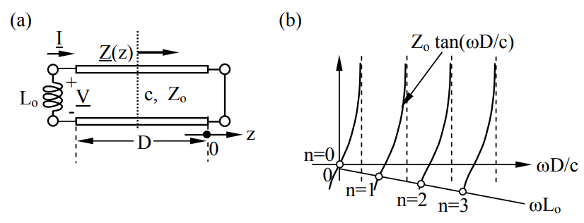
If a TEM resonator is terminated with a reactive impedance such as jωL or 1/jωC, then energy is still trapped but the resonant frequencies are non-uniformly distributed. Figure 7.4.2(a) illustrates a lossless short-circuited TEM line of length D that is terminated with an inductor L_o. Boundary conditions immediately yield an expression for the resonant frequencies ω_n. The impedance of the inductor is jωL_o and that of the TEM line follows from (7.3.6) for Z_L = 0:

\[ \underline{Z}(\mathrm{z})=\mathrm{Z}_{0}\left(\underline{\mathrm{Z}}_{\mathrm{L}}-\mathrm{j} \mathrm{Z}_{\mathrm{o}} \tan \mathrm{kz}\right) /\left(\underline{\mathrm{Z}}_{\mathrm{o}}-\mathrm{j} \mathrm{Z}_{\mathrm{L}} \tan \mathrm{k} \mathrm{z}\right)=-\mathrm{j} \mathrm{Z}_{\mathrm{o}} \tan \mathrm{kz}\]

Since the current \(\underline{\mathrm I} \) and voltage \(\underline{\mathrm V} \) at the inductor junction are the same for both the transmission line and the inductor, their ratios must also be the same except that we define \(\underline{\mathrm I}\) to be flowing out of the inductor into the TEM line, which changes the sign of +jωL_o; so:

\[\underline{V} / \underline{I}=-j \omega L_{0}=j Z_{0} \tan k D \]

\[ \omega_{\mathrm{n}}=-\frac{\mathrm{Z}_{\mathrm{o}}}{\mathrm{L}_{\mathrm{o}}} \tan \mathrm{kD}=-\frac{\mathrm{Z}_{\mathrm{o}}}{\mathrm{L}_{\mathrm{o}}} \tan \left(\omega_{\mathrm{n}} \mathrm{D} / \mathrm{c}\right)>0\]

The values of ω_n that satisfy (7.4.25) are represented graphically in Figure 7.4.2(b), and are spaced non-uniformly in frequency. The resonant frequency ω_o = 0 corresponds to direct current and pure magnetic energy storage. Figure 7.4.2(b) yields ω_n for a line shorted at both ends when L_o = 0, and shows that for small values of L_o (perturbations) that the shift in resonances \(\delta\)ω_n are linear in L_o.

We generally can tune resonances to nearby frequencies by changing the resonator slightly. Section 9.4.2 derives the following expression (7.4.26) for the fractional change \(\delta\)f/f in any resonance f as a function of the incremental increases in average electric (\(\delta\)ω_e) and magnetic

(\(\delta\)ω_m) energy storage and, equivalently, in terms of the incremental volume that was added to or subtracted from the structure, where W_e and W_m are the electric and magnetic energy densities in that added (+\(\delta\)v_vol) or removed (-\(\delta\)v_vol) volume, and w_T is the total energy associated with f. The energy densities can be computed using the unperturbed values of field strength to obtain approximate answers.

\[\Delta \mathrm{f} / \mathrm{f}=\left(\Delta \mathrm{w}_{\mathrm{e}}-\Delta \mathrm{w}_{\mathrm{m}}\right) / \mathrm{w}_{\mathrm{T}}=\Delta \mathrm{v}_{\mathrm{vol}}\left(\mathrm{W}_{\mathrm{e}}-\mathrm{W}_{\mathrm{m}}\right) / \mathrm{w}_{\mathrm{T}} \qquad \qquad \qquad \text { (frequency perturbation) }\]

A simple example illustrates its use. Consider the TEM resonator of Figure 7.4.2(a), which is approximately short-circuited at the left end except for a small tuning inductance L_o having an impedance \(|j \omega L|<<Z_{0}\). How does L_o affect the resonant frequency f₁? One approach is to use (7.4.25) or Figure 7.4.2(b) to find w_n. Alternatively, we may use (7.4.26) to find \( \Delta \mathrm{f}=-\mathrm{f}_{1} \times \Delta \mathrm{w}_{\mathrm{m}} / \mathrm{w}_{\mathrm{T}}\), where \(\mathrm{f}_{1} \cong \mathrm{c} / \lambda \cong \mathrm{c} / 2 \mathrm{D}\) and \(\Delta \mathrm{w}_{\mathrm{m}}=\mathrm{L}_{\mathrm{o}}\left|\mathrm{\underline I}^{\prime}\right|^{2} / 4=\left|\mathrm{\underline V}^{\prime}\right|^{2} / 4 \omega^{2} \mathrm{L}\), where \(\underline {\mathrm{I}}^{\prime}\) and \(\underline {\mathrm{V}}^{\prime}\) are exact. But the unperturbed voltage at the short-circuited end of the resonator is zero, so we must use \(\underline {\mathrm{I}}^{\prime}\) because perturbation techniques require that only small fractional changes exist in parameters to be computed, and a transition from zero to any other value is not a perturbation. Therefore \(\Delta \mathrm{w}_{\mathrm{m}} =\mathrm{L}_{\mathrm{o}}\left|\mathrm{\underline I}_{\mathrm{o}}\right|^{2} / 4\). To cancel \(\left|\underline{\mathrm{I}}_{\mathrm{o}}\right|^{2}\) in the expression for \(\delta\)f, we compute w_T in terms of voltage: \(\mathrm{w}_{\mathrm{T}}=2 \mathrm{w}_{\mathrm{m}}=2 \int_{0}^{\mathrm{D}}\left(\mathrm{L}|\mathrm{\underline I}(\mathrm{z})|^{2} / 4\right) \mathrm{d} \mathrm{z}=\mathrm{D} \mathrm{L} \mathrm{I}_{\mathrm{o}}^{2} / 4\). Thus:

\[\Delta \mathrm{f}=\Delta \mathrm{f}_{\mathrm{n}}=-\mathrm{f}_{\mathrm{n}}\left(\frac{\Delta \mathrm{w}_{\mathrm{m}}}{\mathrm{w}_{\mathrm{T}}}\right)=-\mathrm{f}_{\mathrm{n}} \frac{\left|\underline{\mathrm{I}}_{\mathrm{o}}\right|^{2} / 4}{\mathrm{D} \mathrm{L}\left|\underline{\mathrm{I}}_{\mathrm{o}}\right|^{2} / 4}=-\mathrm{f}_{\mathrm{n}} \frac{\mathrm{L}_{\mathrm{o}}}{\mathrm{LD}}\]

Resonator losses and Q

All resonators dissipate energy due to resistive losses, leakage, and radiation. Since dissipation is proportional to resonator energy content and to the squares of current or voltage, the decay of field strength and stored energy is generally exponential in time. Each resonant frequency f_n has its own rate of energy decay, characterized by the dimensionless quality factor Q_n, which is generally the number of radians ω_nt required for the total energy w_Tn stored in mode n to decay by a factor of 1/e:

\[\mathrm{w}_{\mathrm{Tn}}(\mathrm{t})=\mathrm{w}_{\mathrm{Tn} 0} \mathrm{e}^{-\omega_{\mathrm{n}} \mathrm{t} / \mathrm{Q}_{\mathrm{n}}}\ [\mathrm J]\]

Q_n is easily related to P_n, the power dissipated by mode n:

\[\mathrm {P_{n} \cong-d w_{T n} / d t=\omega_{n} w_{T n} / Q_{n} \ [W] }\]

\[\mathrm{Q}_{\mathrm{n}} \cong \omega_{\mathrm{n}} \mathrm{w}_{\mathrm{Tn}} / \mathrm{P}_{\mathrm{n}} \qquad \qquad \qquad \text{(quality factor Q) }\]

The rate of decay for each mode depends on the location of the resistive or radiating elements relative to the peak currents or voltages for that mode. For example, if a resistive element experiences a voltage or current null, there is no dissipation. These relations apply to all resonators, for example, RLC resonators: (3.5.20–23).

Whether a resonator is used as a band-pass or band-stop filter, it has a bandwidth \(\delta\)ω within which more than half the peak power is passed or stopped, respectively. This half-power bandwidth \(\delta\)ω is simply related to Q by (3.5.36):

\[\mathrm{Q}_{\mathrm{n}} \cong \omega_{\mathrm{n}} / \Delta \omega_{\mathrm{n}}\]

The concept and utility of Q and the use of resonators in circuits are developed further in Section 7.4.4.

Loss in TEM lines arises because the wires are resistive or because the medium between the wires conducts slightly. In addition, lumped resistances may be present, as suggested in Figure 7.4.3(b) and (d). If these resistances do not significantly perturb the lossless voltage and current distributions, then the power dissipated and Q of each resonance ω_n can be easily estimated using perturbation techniques. The perturbation method simply involves computing power dissipation using the voltages or currents appropriate for the lossless case under the assumption that the fractional change induced by the perturbing element is small (perturbations of zero-valued parameters are not allowed). The examples below illustrate that perturbing resistances can be either very large or very small.

Figure \(\PageIndex{3}\): TEM resonators perturbed by loss.

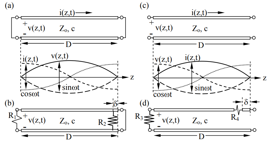
Consider first the illustrated ω₁ resonance of Figure 7.4.3(a) as perturbed by the small resistor R₁ << Z_o; assume R₂ is absent. The nominal current on the TEM line is:

\[\mathrm{i(t, z)=R_{e}\left\{\underline{I} e^{j \omega t}\right\}=I_{o} \sin \omega t \cos (\pi z / D)}\]

The power P₁ dissipated in R₁ at z = 0 using the unperturbed current is:

\[\mathrm{P}_{1}=\left\langle\mathrm{i}^{2}(\mathrm{t}, \mathrm{z}=0)\right\rangle \mathrm{R}_{1}=\mathrm{I}_{\mathrm{o}}^{2} \mathrm{R}_{1} / 2\]

The corresponding total energy w_T1 stored in this unperturbed resonance is twice the magnetic energy:

\[\mathrm{w}_{\mathrm{Tl}}=2 \int_{0}^{\mathrm{D}}\left(\mathrm{L}\left\langle\mathrm{i}^{2}(\mathrm{t})\right\rangle / 2\right) \mathrm{dz}=\mathrm{D} \mathrm{LI}_{\mathrm{o}}^{2} / 4 \ [\mathrm{J}]\]

Using (7.4.30) for Q and (7.4.5) for ω we find:

\[\mathrm{Q}_{1} \cong \omega_{1} \mathrm{w}_{\mathrm{Tl}} / \mathrm{P}_{1}=(\pi \mathrm{c} / \mathrm{D})\left(\mathrm{D} \mathrm{L}_{\mathrm{o}}^{2} / 4\right) /\left(\mathrm{I}_{\mathrm{o}}^{2} \mathrm{R}_{1} / 2\right)=\pi \mathrm{c} \mathrm{L} / 2 \mathrm{R}_{1}=\left(\mathrm{Z}_{\mathrm{o}} / \mathrm{R}_{1}\right) \pi / 2\]

Thus \(\mathrm{Q}_{1} \cong \mathrm{Z}_{0} / \mathrm{R}_{1} \) and is high when R₁ << Z_o; in this case R₁ is truly a perturbation, so our solution is valid.

A more interesting case involves the loss introduced by R₂ in Figure 7.4.3(b) when R₁ is zero. Since the unperturbed shunting current at that position on the line is zero, we must use instead the unperturbed voltage v(z,t) to estimate P₁ for mode 1, where that nominal line voltage is:

\[\mathrm{v}(\mathrm{z}, \mathrm{t})=\mathrm{V}_{0} \sin \omega \mathrm{t} \sin (\pi \mathrm{z} / \mathrm{D})\]

The associated power P₁ dissipated at position \(\delta\), and total energy w_T1 stored are:

\[\mathrm{P}_{1} \cong\left\langle\mathrm{v}(\delta, \mathrm{t})^{2}\right\rangle / \mathrm{R}_{2}=\mathrm{V}_{\mathrm{o}}^{2} \sin ^{2}(\pi \delta / \mathrm{D}) / 2 \mathrm{R}_{2} \cong\left(\mathrm{V}_{\mathrm{o}} \pi \delta / \mathrm{D}\right)^{2} / 2 \mathrm{R}_{2} \ [\mathrm{W}]\]

\[\mathrm{w}_{\mathrm{Tl}} \cong 2 \int_{0}^{\mathrm{D}}\left(\mathrm{C}\left\langle\mathrm{v}^{2}(\mathrm{z}, \mathrm{t})\right\rangle \big/ 2\right) \mathrm{d} \mathrm{z}=\mathrm{D} \mathrm{CV}_{\mathrm{o}}^{2} \big/ 4 \ [\mathrm{J}]\]

Note that averaging v² (z,t) over space and time introduces two factors of 0.5. Using (7.4.35) for Q and (7.4.5) for ω we find:

\[\mathrm{Q}_{1} \cong \omega_{1} \mathrm{w}_{\mathrm{T} 1} / \mathrm{P}_{1}=(\pi \mathrm{c} / \mathrm{D})\left(\mathrm{DCV}_{\mathrm{o}}^{2} / 4\right) \Big/\left[\left(\mathrm{V}_{\mathrm{o}} \pi \delta / \mathrm{D}\right)^{2} \big/ 2 \mathrm{R}_{2}\right]=(\mathrm{D} / \mathrm{\delta})^{2}\left(\mathrm{R}_{2} / 2 \pi \mathrm{Z}_{\mathrm{o}}\right)\]

Thus Q₁ is high and R₂ is a small perturbation if D >> \(\delta\), even if R₂ < Z_o. This is because a leakage path in parallel with a nearby short circuit can be a perturbation even if its conductance is fairly high.

In the same fashion Q can be found for the loss perturbations of Figure 7.4.3(d). For example, if R₄ = 0, then [following (7.4.39)] the effect of R₃ is:

\[\mathrm{Q}_{1} \cong \omega_{1} \mathrm{w}_{\mathrm{T} 1} / \mathrm{P}_{1}=(\pi \mathrm{c} / \mathrm{D})\left(\mathrm{D} \mathrm{C} \mathrm{V}_{\mathrm{o}}^{2} \big/ 4\right) \Big/\left(\mathrm{v}_{\mathrm{o}}^{2} \big/ 2 \mathrm{R}_{3}\right)=(\pi / 2)\left(\mathrm{R}_{3} / \mathrm{Z}_{\mathrm{o}}\right)\]

In this case R₃ is a perturbation if R₃ >> Z_o. Most R₄ values are also perturbations provided \(\delta\) << D, similar to the situation for R₂, because any resistance in series with a nearby open circuit will dissipate little power because the currents there are so small.

Example \(\PageIndex{A}\)

What is the Q of a TEM resonator of length D characterized by ω_o, C, and G?

Solution

Equation (7.4.40) says \(\mathrm{Q}=\omega_{\mathrm{o}} \mathrm{w}_{\mathrm{T}} / \mathrm{P}_{\mathrm{d}}\), where the power dissipated is given by (7.1.61): \(\mathrm{P}_{\mathrm{d}}=\int_{0}^{\mathrm{D}}\left(\mathrm{G}|\mathrm{\underline V}(\mathrm{z})|^{2} / 2\right) \mathrm{dz}\). The total energy stored w_T is twice the average stored electric energy \(\mathrm{w}_{\mathrm{T}}=2 \mathrm{w}_{\mathrm{e}}=2 \int_{0}^{\mathrm{D}}\left(\mathrm{C}|\underline{\mathrm{V}}(\mathrm{z})|^{2} / 4\right) \mathrm{dz}\) [see 7.1.32)]. The voltage distribution \(|\underline{V}(z)|\) in the two integrals cancels in the expression for Q, leaving Q = 2ω_oC/G.

Coupling to resonators

Depending on how resonators are coupled to circuits, they can either pass or stop a band of frequencies of width ~\(\delta\)ω_n centered on a resonant frequency ω_n. This effect can be total or partial; that is, there might be total rejection of signals either near resonance or far away, or only a partial enhancement or attenuation. This behavior resembles that of the series and parallel RLC resonators discussed in Section 3.5.2.

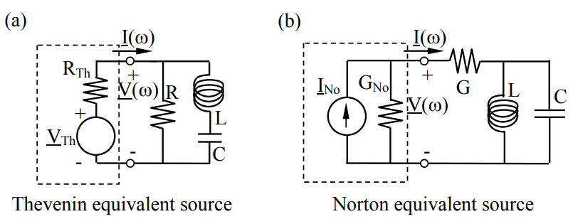
Figure 7.4.4 shows how both series and parallel RLC resonators can block all the available power to the load resistor R_L near resonance, and similar behavior can be achieved with TEM resonators as suggested below; these are called band-stop filters. Alternatively, both series and parallel RLC resonators can pass to the load resistor the band near resonance, as suggested in Figure 3.5.3; these are called band-pass filters. In Figure 7.4.4(a) the series LC resonator shorts out the load R near resonance, while in (b) the parallel LC resonator open-circuits the load conductance G; the resonant band is stopped in both cases.

Figure \(\PageIndex{4}\): CBand-stop RLC resonators.

The half-power width \(\delta\)ω of each resonance is inversely proportional to the loaded Q, where Q_L was defined in (3.5.40), P_DE is the power dissipated externally (in the source resistance R_Th), and P_DI is the power dissipated internally (in the load R):

\[\mathrm{Q}_{\mathrm{L}} \equiv \omega \mathrm{w}_{\mathrm{T}} /\left(\mathrm{P}_{\mathrm{DI}}+\mathrm{P}_{\mathrm{DE}}\right) \qquad \qquad \qquad \text{(loaded Q)}\]

\[\Delta \omega_{\mathrm{n}}=\omega_{\mathrm{n}} / \mathrm{Q}_{\mathrm{n}}\left[\text { radians } \mathrm{s}^{-1}\right] \qquad \qquad \qquad \text{(half-power bandwidth)}\]

When ω = (LC)^-0.5 the LC resonators are either open- or short-circuit, leaving only the source and load resistors, R_Th and R_L. At the frequency f of maximum power transfer the fraction of the available power that can be passed to the load is determined by the ratio Z_n' = R_L/R_Th. For example, if the power source were a TEM transmission line of impedance Z_o ≡ R_Th, then the minimum fraction of incident power reflected from the load (7.2.22) would be:

\[\mathrm{|\underline{\Gamma}|^{2}=\mid\left(\underline{Z}_{n}^{\prime}-1\right) /\left(\underline{Z}_{n}^{\prime}+1\right)^{2}}\]

The fraction reflected is zero only when the normalized load resistance Z_n' = 1, i.e., when R_L = R_Th. Whether the maximum transfer of power to the load occurs at resonance ω_n (band-pass filter) or only at frequencies removed more than ~\(\delta\)ω from ωn (band-stop filter) depends on whether the current is blocked or passed at ω_n by the LC portion of the resonator. For example, Figures 3.5.3 and 7.4.4 illustrate two forms of band-pass and band-stop filter circuits, respectively.

Resonators can be constructed using TEM lines simply by terminating them at both ends with impedances that reflect most or all incident power so that energy remains largely trapped inside, as illustrated in Figure 7.4.5(a). Because the load resistance R_L is positioned close to a short circuit (\(\delta\) << λ/4), the voltage across R_L is very small and little power escapes, even if R_L ≅ Z_o. The Q for the ω₁ resonance is easily calculated by using (7.4.40) and the expression for line voltage (7.4.36):

\[\mathrm{v}(\mathrm{z}, \mathrm{t})=\mathrm{V}_{\mathrm{o}} \sin \omega \mathrm{t} \sin (\pi \mathrm{z} / \mathrm{D})\]

\[\begin{align}\mathrm{Q} & \equiv \omega_{1} \mathrm{w}_{\mathrm{T}} / \mathrm{P}_{\mathrm{D}}=(\pi \mathrm{c} / \mathrm{D})\left(\mathrm{DCV}_{\mathrm{o}}^{2} / 4\right) /\left[\mathrm{v}_{\mathrm{o}}^{2} \sin ^{2}(\pi \delta / \mathrm{D}) / 2 \mathrm{R}_{\mathrm{L}}\right] \nonumber \\&=\left(\pi \mathrm{R}_{\mathrm{L}} / 2 \mathrm{Z}_{\mathrm{o}}\right) / \sin ^{2}(\pi \delta / \mathrm{D}) \cong(\mathrm{D} / \mathrm{s})^{2} \mathrm{R}_{\mathrm{L}} / 2 \pi \mathrm{Z}_{\mathrm{o}} \ \ (\text { for } \delta<<\mathrm{D})\end{align}\]

Adjustment of \(\delta\) enables achievement of any desired Q for any given R_L in an otherwise lossless system. If we regard R_L as internal to the resonator then the Q calculated above is the internal Q, Q_I.

Figure \(\PageIndex{5}\): Coupled TEM resonator.

We may connect this resonator externally by adding a feed line at a short distance \(\delta_{2}\) and from its left end, as illustrated in Figure 7.4.5(b). If the feed line is matched at its left end then the external Q, Q_E, associated with power dissipated there is given by (7.4.45) for \(\delta=\delta_{2}\) and R_L = Z_o. By adjusting \(\delta_{2}\) any Q_E can be obtained. Figures 3.5.3 and 7.4.4 suggest how the equivalent circuits for either band-pass or band-stop filters can match all the available power to the load if R_Th = R_L and therefore Q_E = Q_I. Thus all the available power can be delivered to R_L in Figure 7.4.5(b) for any small \(\delta_{1}\) by selecting \(\delta_{2}\) properly; if \(\delta_{2}\) yields a perfect match at resonance, we have a critically coupled resonator. If \(\delta_{2}\) is larger than the critically coupled value, then the input transmission line is too strongly coupled, Q_E < Q_I, and we have an over-coupled resonator; conversely, smaller values of \(\delta_{2}\) yield Q_E > Q_I and undercoupling. The bandwidth of this bandpass filter \(\delta\)ω is related to the loaded Q, Q_L, as defined in (7.4.41) where:

\[\mathrm{\mathrm{Q}_{\mathrm{L}}^{-1}=\mathrm{Q}_{\mathrm{I}}^{-1}+\mathrm{Q}_{\mathrm{E}}^{-1}}=\Delta \omega / \omega\]

If the band-pass filter of Figure 7.4.5(b) is matched at resonance so Q_E = Q_I, it therefore has a bandwidth \(\delta\)ω = 2ω/Q_I, where Q_I is given by (7.4.39) and is determined by our choice of \(\delta_{1}\). Smaller values of \(\delta_{1}\) yield higher values for Q_L and narrower bandwidths \(\delta\)ω. In the special case where R_L corresponds to another matched transmission line with impedance Z_o, then a perfect match at resonance results here when \(\delta_{1}=\delta_{2}\).

Many variations of the coupling scheme in Figure 7.4.5 exist. For example, the feed line and resonator can be isolated by a shunt consisting of a large capacitor or a small inductor, both approximating short circuits relative to Z_o, or by a high-impedance block consisting of a small capacitor or large inductor in series. Alternatively, an external feed line can be connected in place of R₄ in Figure 7.4.3(d). In each weakly coupled case perturbation methods quickly yield Q_I and Q_E, and therefore Q_L, \(\delta\)ω, and the impedance at resonance.

The impedance at resonance can be found once Q_E, Q_I, and Z_o for the feedline are known, and once it is known whether the resonance is a series or parallel resonance. Referring to Figures 3.5.3 and 7.4.4 for equivalent circuits for band-pass and band-stop filters, respectively, it is clear that if Q_E = Q_I, then band-pass resonators are matched at resonance while band-stop series-resonance resonators are short circuits and parallel-resonance resonators are open circuits. Away from resonance band-pass resonators become open circuits for series resonances and short circuits for parallel resonances, while both types of band-stop resonator become matched loads if Q_E = Q_I. At resonance all four types of resonator have purely real impedances and reflection coefficients \(\Gamma\) that can readily be found by examining the four equivalent circuits cited above.

Sometimes unintended resonances can disrupt systems. For example, consider a waveguide that can propagate two modes, only one of which is desired. If a little bit of the unwanted mode is excited at one end of the waveguide, but cannot escape through the lines connected at each end, then the second mode is largely trapped and behaves as a weakly coupled resonator with its own losses. At each of its resonances it will dissipate energy extracted from the main waveguide. If the internal losses happen to cause Q_E = Q_I for these parasitic resonances, no matter how weakly coupled they are, they can appear as a matched load positioned across the main line; dissipation by parasitic resonances declines as their internal and external Q’s increasingly differ.

The ability of a weakly coupled resonance to have a powerful external effect arises because the field strengths inside a low-loss resonator can rise to values far exceeding those in the external circuit. For example, the critically coupled resonator of Figure 7.4.5(b) for R_L = Z_o and \(\delta_{1}=\delta_{2}\), has internal voltages v(z,t) = V_osinωt sin(\(\pi\)z/D) given by (7.4.44), where the maximum terminal voltage is only \(\mathrm{V}_{\mathrm{o}} \sin (\pi \delta / \mathrm{D}) \cong \mathrm{V}_{\mathrm{o}} \pi \delta / \mathrm{D}<<\mathrm{V}_{\mathrm{o}}\). Thus a parasitic resonance can slowly absorb energy from its surroundings at its resonant frequency until its internal fields build to the point that even with weak coupling it has a powerful effect on the external fields and thus reaches an equilibrium value. It is these potentially extremely strong resonant fields that enables critically coupled resonators to couple energy into poorly matched loads--the fields in the resonator build until the power dissipated in the load equals the available power provided. In some cases the fields can build to the point where the resonator arcs internally, as can happen with an empty microwave oven without an extra internal load to prevent it.

This analysis of the resonant behavior of TEM lines is approximate because the resonator length measured in wavelengths is a function of frequency within \(\delta\)ω, so exact answers require use the TEM analysis methods of Sections 7.2–3, particularly when \(\delta\)ω becomes a non-trivial fraction of the frequency difference between adjacent resonances.

Example \(\PageIndex{B}\)

Consider a variation of the coupled resonator of Figure 7.4.5(b) where the resonator is opencircuited at both ends and the weakly coupled external connections at \(\delta_{1}\) and \(\delta_{2}\) from the ends are in series with the 100-ohm TEM resonator line rather than in parallel. Find \(\delta_{1}\) and \(\delta_{2}\) for: Q_L = 100, Z_o = 100 ohms for both the feed line and resonator, R_L = 50 ohms, and the resonator length is D ≅ λ/2, where λ is the wavelength within the resonator.

Solution

For critical coupling, Q_E = Q_I, so the resonator power lost to the input line, \(\left|\mathrm{\underline I}_{2}\right|^{2} \mathrm{Z}_{\mathrm{o}} / 2\), must equal that lost to the load, \(\left|\mathrm{\underline I}_{2}\right|^{2} \mathrm{R}_{2} / 2\), and therefore \(\left|\mathrm{\underline I}_{1}\right| /\left|\underline{\mathrm{I}}_{2}\right| = \mathrm{\left(Z_{0} / R_{L}\right)^{0.5}}=2^{0.5}\). Since the λ/2 resonance of an open-circuited TEM line has I(z) ≅ I_o sin(\(\pi\)z/D) ≅ \(\pi\)z/D for \(\delta<<\mathrm{D} / \pi\) (high Q), therefore \(\mathrm{\left|\underline{I}_{1}\right| /\left|\underline{I}_{2}\right|=\left[\sin \left(\pi \delta_{1} / D\right)\right] /\left[\sin \left(\pi \delta_{2} / D\right)\right]} \cong \delta_{1} / \delta_{2} \cong 2^{0.5}\). Also, Q_L=100=0.5×Q_I=0.5ω_ow_T/P_DI, where: ω_o=2\(\pi\)f_o=2\(\pi\)c/λ=\(\pi\)c/D; \(\mathrm{w}_{\mathrm{T}}=2 \mathrm{w}_{\mathrm{m}}=2 \int_{0}^{\mathrm{D}}\left(\mathrm{L}|\mathrm{I}|^{2} / 4\right) \mathrm{d} \mathrm{z} \cong \mathrm{L} \mathrm{I}_{\mathrm{o}}^{2} \mathrm{D} / 4\); and \(\mathrm{P}_{\mathrm{DI}}=\left|\mathrm{I}\left(\delta_{1}\right)\right|^{2} \mathrm{R}_{\mathrm{L}} / 2= \mathrm{I}_{\mathrm{o}}^{2} \sin ^{2}\left(\pi \delta_{1} / \mathrm{D}\right) \mathrm{R}_{\mathrm{L}} / 2 \cong\left(\mathrm{I}_{\mathrm{o}} \pi \delta_{1} / \mathrm{D}\right)^{2} \mathrm{R}_{\mathrm{L}} / 2\). Therefore

\[\mathrm{Q}_{\mathrm{I}}=\omega_{\mathrm{o}} \mathrm{W}_{\mathrm{T}} / \mathrm{P}_{\mathrm{DI}}=200= (\pi \mathrm{c} / \mathrm{D})\left(\mathrm{LI}_{\mathrm{o}}^{2} \mathrm{D} / 4\right) /\left[\left(\mathrm{I}_{\mathrm{o}} \pi \delta_{1} / \mathrm{D}\right)^{2} \mathrm{R}_{\mathrm{L}} / 2\right]=\left(\mathrm{D} / \delta_{1}\right)^{2}\left(\mathrm{Z}_{\mathrm{o}} / \mathrm{R}_{\mathrm{L}}\right) / \pi,\nonumber\]

where cL = Z_o = 100. Thus \(\delta_{1}=\pi^{-0.5} \mathrm{D} / 10\) and \(\delta_{2}=\delta_{1} 2^{-0.5}=(2 \pi)^{-0.5} \mathrm{D} / 10\).

Transients in TEM resonators

TEM and cavity resonators have many resonant modes, all of which can be energized simultaneously, depending on initial conditions. Because Maxwell’s equations are linear, the total fields can be characterized as the linear superposition of fields associated with each excited mode. This section illustrates how the relative excitation of each TEM resonator mode can be determined from any given set of initial conditions, e.g. from v(z, t = 0) and i(z, t = 0), and how the voltage and current subsequently evolve. The same general method applies to modal excitation of cavity resonators. By using a similar orthogonality method to match boundary conditions in space rather than in time, the modal excitation of waveguides and optical fibers can be found, as discussed in Section 9.3.3.

The central concept developed below is that any initial condition in a TEM resonator at time zero can be replicated by superimposing some weighted set of voltage and current modes. Once the phase and magnitudes of those modes are known, the voltage and current are then known for all time. The key solution step uses the fact that the mathematical functions characterizing any two different modes a and b, e.g. the voltage distributions \(\mathrm{\underline{V}_{a}(z)}\) and \(\mathrm{\underline{V}_{b}(z)}\), are spatially othogonal: \(\int \underline{V}_{\mathrm{a}}(\mathrm{z}) \underline{\mathrm{V}}_{\mathrm{b}} *(\mathrm{z}) \mathrm{d} \mathrm{z}=0\).

Consider the open-circuited TEM resonator of Figure 7.4.3(c), for which \(\underline{V}_{n-}=\underline{V}_{n+}\) for any mode n because the reflection coefficient at the open circuit at z = 0 is +1. The resulting voltage and current on the resonator for mode n are:³⁹

³⁹ Where we recall \(\cos \phi=\left(\mathrm{e}^{\mathrm{j} \phi}+\mathrm{e}^{-\mathrm{j} \phi}\right) / 2\) and \(\sin \phi=\left(\mathrm{e}^{\mathrm{j} \phi}-\mathrm{e}^{-\mathrm{j} \phi}\right) / 2 \mathrm{j}\).

\[\mathrm{\underline{V}_{n}(z)=\underline{V}_{n+} \mathrm{e}^{-j k_{n} z}+\underline{V}_{n-} e^{+j k_{n} z}=2 \underline{V}_{n+} \cos k_{n} z}\]

\[\mathrm{\underline{I}_{n}(z)=Y_{0}\left(\underline{V}_{n+} e^{-j k_{n} z}-\underline{V}_{n-} e^{+j k_{n} z}\right)=-2 j Y_{0} \underline{V}_{n+} \sin k_{n} z}\]

where k_n = ω_n/c and (7.4.5) yields ω_n = n\(\pi\)c/D. We can restrict the general expressions for voltage and current to the moment t = 0 when the given voltage and current distributions are v_o(z) and i_o(z):

\[\left.\mathrm{v}(\mathrm{z}, \mathrm{t}=0)=\mathrm{v}_{0}(\mathrm{z})=\sum_{\mathrm{n}=0}^{\infty} \mathrm{R}_{\mathrm{e}}\left\{\mathrm{\underline V}_{\mathrm{n}}(\mathrm{z}) \mathrm{e}^{\mathrm{j} \omega_{\mathrm{n}} \mathrm{t}}\right\}_{\mathrm{t}=0}=\sum_{\mathrm{n}=0}^{\infty} \mathrm{R}_{\mathrm{e}}\left\{2 \underline{\mathrm{V}}_{\mathrm{n}+} \cos \mathrm{k}_{\mathrm{n}}\mathrm{z}\right\}\right\}\]

\[\mathrm{i(z, t=0)=i_{0}(z)=\sum_{n=0}^{\infty} R_{e}\left\{\underline I_{n}(z) e^{j \omega_{n} t}\right\}_{t=0}=Y_{0} \sum_{n=0}^{\infty} I_{m}\left\{2 \underline{V}_{n+} \sin k_{n} z\right\}}\]

We note that these two equations permit us to solve for both the real and imaginary parts of \(\mathrm {\underline{V}_{n+}}\), and therefore for v(z,t) and i(z,t). Using spatial orthogonality of modes, we multiply both sides of (7.4.49) by cos(m\(\pi\)z/D) and integrate over the TEM line length D, where k_n = n\(\pi\)z/D:

\[\begin{align}&\int_{0}^{\mathrm{D}} \mathrm{v}_{\mathrm{o}}(\mathrm{z}) \cos (\mathrm{m} \pi \mathrm{z} / \mathrm{D}) \mathrm{d} \mathrm{z}=\int_{0}^{\mathrm{D}} \sum_{\mathrm{n}=0}^{\infty} \mathrm{R}_{\mathrm{e}}\left\{2 \underline{\mathrm{V}}_{\mathrm{n}+} \cos \mathrm{k}_{\mathrm{n}} \mathrm{z}\right\} \cos (\mathrm{m} \pi \mathrm{z} / \mathrm{D}) \mathrm{d} \mathrm{z} \nonumber \\&\quad=\sum_{\mathrm{n}=0}^{\infty} \mathrm{R}_{\mathrm{e}}\left\{2 \underline{\mathrm{V}}_{\mathrm{n}+}\right\} \int_{0}^{\mathrm{D}} \cos (\mathrm{n} \pi \mathrm{z} / \mathrm{D}) \cos (\mathrm{m} \pi \mathrm{z} / \mathrm{D}) \mathrm{d} \mathrm{z}=2 \mathrm{R}_{\mathrm{e}}\left\{\mathrm{V}_{\mathrm{n}+}\right\}(\mathrm{D} / 2) \delta_{\mathrm{mn}}\end{align}\]

where \(\delta_{\mathrm{mn}} \equiv 0 \) if m ≠ n, and \(\delta_{\mathrm{mn}} \equiv 1 \) if m = n. Orthogonality of modes thus enables this integral to single out the amplitude of each mode separately, yielding:

\[\mathrm{R}_{\mathrm{e}}\left\{\mathrm{\underline V}_{\mathrm{n}+}\right\}=\mathrm{D}^{-1} \int_{0}^{\mathrm{D}} \mathrm{v}_{\mathrm{o}}(\mathrm{z}) \cos (\mathrm{n} \pi \mathrm{z} / \mathrm{D}) \mathrm{d} \mathrm{z}\]

Similarly, we can multiply (7.4.50) by sin(m\(\pi\)z/D) and integrate over the length D to yield:

\[\operatorname{Im}\left\{\underline{\mathrm{V}}_{\mathrm{n}+}\right\}=\mathrm{Z}_{\mathrm{o}} \mathrm{D}^{-1} \int_{0}^{\mathrm{D}} \mathrm{i}_{\mathrm{o}}(\mathrm{z}) \sin (\mathrm{n} \pi \mathrm{z} / \mathrm{D}) \mathrm{dz}\]

Once \(\mathrm{\underline{V}_{n}}\) is known for all n, the full expressions for voltage and current on the TEM line follow, where ω_n = \(\pi\)nc/D:

\[\mathrm{v}(\mathrm{z}, \mathrm{t})=\sum_{\mathrm{n}=0}^{\infty} \mathrm{R}_{\mathrm{e}}\left\{\underline{\mathrm{V}}_{\mathrm{n}}(\mathrm{z}) \mathrm{e}^{\mathrm{j} \omega_{\mathrm{n}} \mathrm{t}}\right\} \]

\[ \mathrm{i(z, t)=\sum_{n=0}^{\infty} R_{e}\left\{\underline I_{n}(z) e^{j \omega_{n} t}\right\}=Y_{o} \sum_{n=0}^{\infty} I_{m}\left\{2_{-} V_{n+} \sin k_{n} z\right\}}\]

In general, each resonator mode decays exponentially at its own natural rate, until only the longest-lived mode remains.

As discussed in Section 9.3.3, the relative excitation of waveguide modes by currents can be determined in a similar fashion by expressing the fields in a waveguide as the sum of modes, and then matching the boundary conditions imposed by the given excitation currents at the spatial origin (not time origin). The real and imaginary parts of the amplitudes characterizing each waveguide propagation mode can then be determined by multiplying both sides of this boundary equation by spatial sines or cosines corresponding to the various modes, and integrating over the surface defining the boundary at z = 0. Arbitrary spatial excitation currents generally excite both propagating and evanescent modes in some combination. Far from the excitation point only the propagating modes are evident, while the evanescent modes are evident principally as a reactance seen by the current source.