9.5: Waves in complex media

Waves in anisotropic media

There are many types of media that can be analyzed simply using Maxwell’s equations, which characterize media by their permittivity ε, permeability μ, and conductivity σ. In general ε, η, and σ can be complex, frequency dependent, and functions of field direction. They can also be functions of density, temperature, field strength, and other quantities. Moreover they can also couple \( \overline{\mathrm{E}}\) to \(\overline{\mathrm{B}}\), \(\overline{\mathrm{H}} \) to \(\overline{\mathrm{D}} \). In this section we only treat the special cases of anisotropic media (Section 9.5.1), dispersive media (Section 9.5.2), and plasmas (Section 9.5.3). Lossy media were treated in Sections 9.2.4 and 9.2.5.

Anisotropic media, by definition, have permittivities, permeabilities, and/or conductivities that are functions of field direction. We can generally represent these dependences by 3×3 matrices (tensors), i.e.:

\[\overline{\mathrm{D}}=\overline{ \overline{\varepsilon}} \overline{\mathrm{E}}\]

\[\overline{\mathrm{B}}=\overline{\overline{\mu}} \ \overline{\mathrm{H}}\]

\[\overline{\mathrm{J}}=\overline{\overline{\sigma}} \ \overline{\mathrm{E}}\]

For example, (9.5.1) says:

\[\begin{array}{l}
\mathrm{D}_{\mathrm{x}}=\varepsilon_{\mathrm{xx}} \mathrm{E}_{\mathrm{x}}+\varepsilon_{\mathrm{xy}} \mathrm{E}_{\mathrm{y}}+\varepsilon_{\mathrm{xz}} \mathrm{E}_{\mathrm{z}} \\
\mathrm{D}_{\mathrm{y}}=\varepsilon_{\mathrm{yx}} \mathrm{E}_{\mathrm{x}}+\varepsilon_{\mathrm{yy}} \mathrm{E}_{\mathrm{y}}+\varepsilon_{\mathrm{yz}} \mathrm{E}_{\mathrm{z}} \\
\mathrm{D}_{\mathrm{z}}=\varepsilon_{\mathrm{zx}} \mathrm{E}_{\mathrm{x}}+\varepsilon_{\mathrm{zy}} \mathrm{E}_{\mathrm{y}}+\varepsilon_{\mathrm{zz}} \mathrm{E}_{\mathrm{z}}
\end{array}\]

Most media are symmetric so that ε_ij = ε_ji; in this case the matrix \(\overline{\overline{\varepsilon}}\) can always be diagonalized by rotating the coordinate system to define new directions x, y, and z that yield zeros off-axis:

\[\overline{\overline{\varepsilon}}=\left(\begin{array}{ccc}\varepsilon_{\mathrm{x}} & 0 & 0 \\0 & \varepsilon_{\mathrm{y}} & 0 \\0 & 0 & \varepsilon_{\mathrm{z}}\end{array}\right)\]

These new axes are called the principal axes of the medium. The medium is isotropic if the permittivities of these three axes are equal, uniaxial if only two of the three axes are equal, and biaxial if all three differ. For example, tetragonal, hexagonal, and rhombohedral crystals are uniaxial, and orthorhombic, monoclinic, and triclinic crystals are biaxial. Most constitutive tensors are symmetric (they equal their own transpose), the most notable exception being permeability tensors for magnetized media like plasmas and ferrites, which are hermetian⁴⁹ and not discussed in this text.

⁴⁹ Hermetian matrices equal the complex conjugate of their transpose.

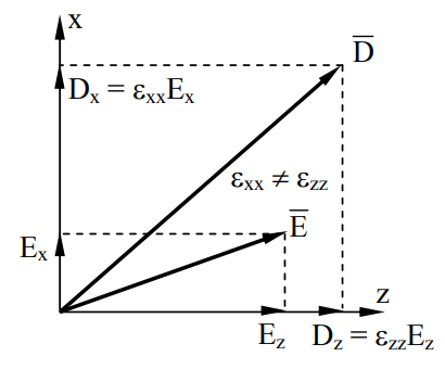
One immediate consequence of anisotropic permittivity and (9.5.4) is that \(\overline{\mathrm D}\) is generally no longer parallel to \(\overline{\mathrm E}\), as suggested in Figure 9.5.1 for a uniaxial medium. When ε_xx ≠ ε_zz, \(\overline{\mathrm E}\) and \(\overline{\mathrm D}\) are parallel only if they lie along one of the principal axes. As explained shortly, this property of uniaxial or biaxial media can be used to convert any wave polarization into any other.

Figure \(\PageIndex{1}\): \(\overline{\mathrm D}\) and \(\overline{\mathrm E}\) in an anisotropic medium.

The origins of anisotropy in media are easy to understand in terms of simple models for crystals. For example, an isotropic cubic lattice becomes uniaxial if it is compressed or stretched along one of those axes, as illustrated in Figure 9.5.2(a) for z-axis compression. That such compressed columns act to increase the effective permittivity in their axial direction can be understood by noting that each of these atomic columns functions like columns of dielectric between capacitor plates, as suggested in Figure 9.5.2(b). Parallel-plate capacitors were discussed in Section 3.1.3. Alternatively the same volume of dielectric could be layered over one of the capacitor plates, as illustrated in Figure 9.5.2(c).

Figure \(\PageIndex{2}\): Uniaxial crystal and anisotropically filled capacitors.

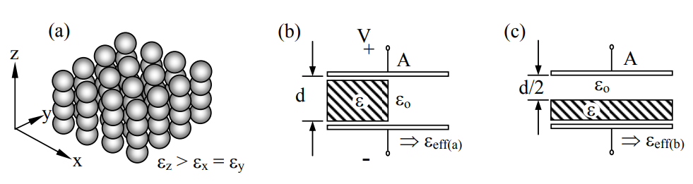
Even though half the volume between the capacitor plates is occupied by dielectric in both these cases, the capacitance for the columns [Figure 9.5.2(b)] is greater, corresponding to a greater effective permittivity \(\varepsilon_{\mathrm{eff}}\). This can be shown using Equation (3.1.10), which says that a parallel plate capacitor has \(\mathrm{C}=\varepsilon_{\mathrm{eff}} \mathrm{A} / \mathrm{d}\), where A is the plate area and d is the distance between the plates. The capacitances C_a and C_b for Figures 9.5.2(b) and (c) correspond to two capacitors in parallel and series, respectively, where:

\[\mathrm{C}_{\mathrm{a}}=(\varepsilon \mathrm{A} / 2 \mathrm{d})+\left(\varepsilon_{\mathrm{o}} \mathrm{A} / 2 \mathrm{d}\right)=\left(\varepsilon+\varepsilon_{\mathrm{o}}\right) \mathrm{A} / 2 \mathrm{d}=\varepsilon_{\mathrm{eff}(\mathrm{a})} \mathrm{A} / \mathrm{d}\]

\[\mathrm{C}_{\mathrm{b}}=\left[(\varepsilon \mathrm{A} 2 / \mathrm{d})^{-1}+\left(\varepsilon_{\mathrm{o}} \mathrm{A} 2 / \mathrm{d}\right)^{-1}\right]^{-1}=\left[\varepsilon \varepsilon_{\mathrm{o}} /\left(\varepsilon+\varepsilon_{\mathrm{o}}\right)\right] 2 \mathrm{A} / \mathrm{d}=\varepsilon_{\mathrm{eff}(\mathrm{b})} \mathrm{A} / \mathrm{d}\]

In the limit where ε >> ε_o the permittivity ratio ε_eff(a)/ ε_eff(b) → ε/4ε_o > 1. In all compressive cases ε_eff(a) ≥ ε_eff(b). If the crystal were stretched rather than compressed, this inequality would be reversed. Exotic complex materials can exhibit inverted behavior, however.

Since the permittivity here interacts directly only with \(\overline{\mathrm{E}}\), not \(\overline{\mathrm{H}}\), the velocity of propagation \(c=1 / \sqrt{\mu \varepsilon}\) depends only on the permittivity in the direction of \(\overline{\mathrm{E}}\). We therefore expect slower propagation of waves linearly polarized so that \(\overline{\mathrm{E}}\) is parallel to an axis with higher values of ε. We can derive this behavior from the source-free Maxwell’s equations and the matrix constitutive relation (9.5.4).

\[\mathrm{\nabla \times \overline{\underline{E}}=-j \omega \mu \overline{\underline{H}}}\]

\[\nabla \times \underline{\mathrm{\overline H}}=\mathrm{j} \omega \underline{\mathrm{\overline D}}\]

\[\nabla \bullet \overline{\underline{\mathrm D}}=0\]

\[\nabla \bullet \overline{\underline{\mathrm B}}=0\]

Combining the curl of Faraday’s law (9.5.8) with Ampere’s law (9.5.9), as we did in Section 2.3.3, yields:

\[\nabla \times(\nabla \times \overline{\mathrm{\underline E}})=\nabla(\nabla \bullet \overline{\mathrm{\underline E}})-\nabla^{2} \overline{\mathrm{\underline E}}=\omega^{2} \mu \overline{\mathrm{\underline D}}\]

We now assume, and later prove, that \(\nabla \bullet \overline{\underline{\mathrm E}}=0 \), so (9.5.12) becomes:

\[\nabla^{2} \overline{\mathrm{\underline E}}+\omega^{2} \mu \overline{\mathrm{\underline D}}=0\]

This expression can be separated into independent equations for each axis. Waves propagating in the z direction are governed by the x and y components of (9.5.13):

\[\left[\left(\partial^{2} / \partial \mathbf{z}^{2}\right)+\omega^{2} \mu \varepsilon_{\mathrm{x}}\right] \underline{\mathrm{E}}_{\mathrm{x}}=0\]

\[\left[\left(\partial^{2} / \partial z^{2}\right)+\omega^{2} \mu \varepsilon_{y}\right] \mathrm{ \underline{E}_{y}}=0\]

The wave equation (9.5.14) characterizes the propagation of x-polarized waves and (9.5.15) characterizes y-polarized waves; their wave velocities are \(\left(\mu \varepsilon_{\mathrm{x}}\right)^{-0.5}\) and \(\left(\mu \varepsilon_{\mathrm{y}}\right)^{-0.5}\), respectively. If ε_x ≠ ε_y then the axis with the lower velocity is called the “slow” axis, and the other is the “fast” axis. This dual-velocity phenomenon is called birefringence. That our assumption \(\nabla \bullet \overline{\mathrm{E}}=0\) is correct is easily seen by noting that the standard wave solution for both x- and y- polarized waves satisfies these constraints. Since ∇ is distributive, the equation is also satisfied for arbitrary linear combinations of x- and y- polarized waves, which is the most general case here.

If a wave has both x- and y-polarized components, the polarization of their superposition will evolve as they propagate along the z axis at different velocities. For example, a linearly wave polarized at 45 degrees to the x and y axes will evolve into elliptical and then circular polarization before evolving back into linear polarization orthogonal to the input.

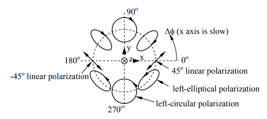
This ability of a birefringent medium to transform polarization is illustrated in Figure 9.5.3. In this case we can represent the linearly polarized wave at z = 0 as:

\[\overline{\mathrm{E}}(\mathrm{z}=0)=\mathrm{E}_{\mathrm{o}}(\hat{x}+\hat{y})\]

If the wave numbers for the x and y axes are k_x and k_y, respectively, then the wave at position z will be:

\[\overline{\mathrm{E}}(\mathrm z)=\mathrm{E}_{\mathrm{o}} e^{-\mathrm{j} \mathrm{k}_{\mathrm{x}} \mathrm{z}}\left(\hat{x}+\hat{y} e^{\mathrm{j}\left(\mathrm{k}_{\mathrm{x}}-\mathrm{k}_{\mathrm{y}}\right) \mathrm{z}}\right)\]

The phase difference between the x- and y-polarized components of the electric field is therefore Δ\(\phi\) = (k_x - k_y)z. As suggested in the figure, circular polarization results when the two components are 90 degrees out of phase (Δ\(\phi\) = ±90^o), and the orthogonal linear polarization results when Δ\(\phi\) = 180^o.

Figure \(\PageIndex{3}\): Polarization conversion in a birefringent medium.

Polarization conversion is commonly used in optical systems to convert linear polarization to circular, or vice-versa, via a quarter-wave plate for which Δ\(\phi\) is 90^o, equivalent to a quarter wavelength. A half-wave plate (Δ\(\phi\) = 180^o) reverses the sense of any polarization.

Example \(\PageIndex{A}\)

A certain birefringent medium is characterized by μ_o, ε_x = 2ε_o, ε_y = 2.002ε_o. How thick D must a quarter-wave plate be if λ = 5×10^-7 [m] in free space (visible light)? At what thickness D' might this same plate rotate appropriate linear polarization 90 degrees?

Solution

The phase lags along the x and y axes arise from \( \mathrm{e}^{-\mathrm{jk}_{\mathrm{x}} \mathrm{D}}\) and \( \mathrm{e}^{-\mathrm{jk}_{\mathrm{y}} \mathrm{D}}\), respectively, and the difference is \(\pi / 2=\left(\mathrm{k}_{\mathrm{y}}-\mathrm{k}_{\mathrm{x}}\right) \mathrm{D} \) for a quarter-wave plate. But \(\mathrm{k}_{\mathrm{i}}=\omega\left(\mu_{\mathrm{o}} \varepsilon_{\mathrm{i}}\right)^{0.5} \), so \(\left(\mathrm{k}_{\mathrm{y}}-\mathrm{k}_{\mathrm{x}}\right) \mathrm{D}=\omega\left(\mu_{\mathrm{o}} \varepsilon_{\mathrm{x}}\right)^{0.5}\left[(1+1.001)^{0.5}-1\right] \mathrm{D} \cong\left(\omega / \mathrm{c}_{\mathrm{x}}\right)^{0.5} 0.0005 \mathrm{D}=\pi / 2 \). Since \( \omega / c_{x}=2 \pi / \lambda_{\mathrm{x}}\), therefore \( D=2000 \lambda_{x} / 4\) where \( \lambda_{\mathrm{x}}=5 \times 10^{-7}\left(\varepsilon_{\mathrm{o}} / \varepsilon_{\mathrm{x}}\right)^{0.5}\). Thus \(D=500 \lambda_{x}=0.18 \) mm, which is approximately the thickness of a Vu-Graph transparency that acts as a quarter-wave plate. A differential phase lag of \(\pi\) yields 90° polarization rotation for waves linearly polarized at an angle 45° from the principal axes x and y, so the thickness would be doubled to ~0.36 mm.

Waves in dispersive media

Dispersive media have wave velocities that are frequency dependent due to the frequency dependence of μ, ε, or σ. These frequency dependencies arise in all materials because of the non-instantaneous physical responses of electrons to fields. Often these time lags are so brief that only at optical frequencies do they become a significant fraction of a period, although propagation over sufficiently long paths can introduce significant cumulative differences in effects across any frequency band or gap. Only vacuum is essentially non-dispersive.

The principal consequence of dispersion is that narrowband pulse signals exhibit two velocities, the phase velocity v_p of the sinusoids within the pulse envelope, and the group velocity v_g at which the pulse envelope, energy, and information propagate. Because energy and information travel at the group velocity, it never exceeds the velocity of light although phase velocity frequently does.

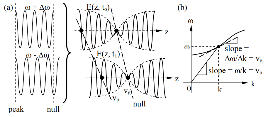
A simple way to reveal this phenomenon is to superimpose two otherwise identical sinusoidal waves propagating at slightly different frequencies, ω ± Δω; superposition is valid because Maxwell’s equations are linear. The corresponding wave numbers are k ± Δk, where Δk << k and Δω << ω. Such a superposition for two sinusoids propagating in the +z direction is:

\[\begin{align}
\mathrm{E}(\mathrm{t}, \mathrm{z}) &=\mathrm{E}_{\mathrm{o}} \cos [(\omega+\Delta \omega) \mathrm{t}-(\mathrm{k}+\Delta \mathrm{k}) \mathrm{z}]+\mathrm{E}_{\mathrm{o}} \cos [(\omega-\Delta \omega \mathrm{t})-(\mathrm{k}-\Delta \mathrm{k}) \mathrm{z}] \nonumber\\
&=\mathrm{E}_{\mathrm{o}} 2 \cos (\omega \mathrm{t}-\mathrm{kz}) \cos (\Delta \omega \mathrm{t}-\Delta \mathrm{kz})
\end{align}\]

where we used the identity \( \cos \alpha+\cos \beta=2 \cos [(\alpha+\beta) / 2] \cos [(\alpha-\beta) / 2]\). The first factor on the right-hand side of (9.5.18) is a sine wave propagating at the center frequency ω at the phase velocity:

\[\mathrm{v}_{\mathrm{p}}=\omega / \mathrm{k} \qquad \qquad \qquad \text{(phase velocity) }\]

The second factor is the low-frequency, long-wavelength modulation envelope that propagates at the group velocity \( \mathrm{v}_{\mathrm{g}}=\Delta \omega / \Delta \mathrm{k}\), which is the slope of the ω(k) dispersion relation:

\[\mathrm{v}_{\mathrm{g}}=\partial \omega / \partial \mathrm{k}=(\partial \mathrm{k} / \partial \omega)^{-1} \qquad \qquad \qquad \text{(group velocity) }\]

Figure 9.5.4(a) illustrates the original sinusoids plus their superposition at two points in time, and Figure 9.5.4(b) illustrates the corresponding dispersion relation.

Figure \(\PageIndex{4}\): Phase and group velocity for two superimposed sinusoids.

Note that this dispersion relation has a phase velocity that approaches infinity at the lowest frequencies, which is what happens in plasmas near the plasma frequency, as discussed in the next section.

Communications systems employ finite-duration pulses with Fourier components at all frequencies, so if such pulses travel sufficiently far even the envelope with its finite bandwidth will become distorted. As a result dispersive media are either avoided or compensated in most communications system unless the bandwidths are sufficiently narrow. Compensation is possible because dispersion is a linear process so inverse filters are readily designed. Section 12.2.2 discusses dispersion further in the context of optical fibers.

Example \(\PageIndex{B}\)

When \( \omega=c_{0}^{0.5}\), what are the phase and group velocities v_p and v_g in a medium having the dispersion relation \(\mathrm{k}=\omega^{2} / \mathrm{c}_{\mathrm{o}} \)?

Solution

\(\mathrm{v}_{\mathrm{p}}=\omega / \mathrm{k}=\mathrm{c}_{\mathrm{o}} / \omega=\mathrm{c}_{\mathrm{o}}^{0.5} \ \left[\mathrm{m} \mathrm{s}^{-1}\right]\). \(\mathrm{v}_{\mathrm{g}}=(\partial \mathrm{k} / \partial \omega)^{-1}=\mathrm{c}_{\mathrm{o}} / 2 \omega=\mathrm{c}_{\mathrm{o}}^{0.5} / 2 \ \left[\mathrm{m} \mathrm{s}^{-1}\right]\).

Waves in plasmas

A plasma is a charge-neutral gaseous assembly of atoms or molecules with enough free electrons to significantly influence wave propagation. Examples include the ionosphere⁵⁰, the sun, interiors of fluorescent bulbs or nuclear fusion reactors, and even electrons in metals or electron pairs in superconductors. We can characterize fields in plasmas once we know their permittivity ε at the frequency of interest.

⁵⁰ The terrestrial ionosphere is a partially ionized layer at altitudes ~50-5000 km, depending primarily upon solar ionization. Its peak electron density is ~10¹² electrons m^-3 at 100-300 km during daylight.

To compute the permittivity of a non-magnetized plasma we recall (2.5.8) and (2.5.13):

\[\overline{\mathrm{D}}=\varepsilon \overline{\mathrm{E}}=\varepsilon_{\mathrm{o}} \overline{\mathrm{E}}+\overline{\mathrm{P}}=\varepsilon_{\mathrm{o}} \overline{\mathrm{E}}+\mathrm{nq} \overline{\mathrm{d}}\]

where q = -e is the electron charge, \(\overline{\mathrm{d}} \) is the mean field-induced displacement of the electrons from their equilibrium positions, and n₃ is the number of electrons per cubic meter. Although positive ions are also displaced, these displacements are generally negligible in comparison to those of the electrons because the electron masses m_e are so much less. We can take the mass m_i of the ions into account simply by replacing m_e in the equations by m_r, the reduced mass of the electrons, where it can be shown that \(\mathrm{m}_{\mathrm{r}}=\mathrm{m}_{\mathrm{e}} \mathrm{m}_{\mathrm{i}} /\left(\mathrm{m}_{\mathrm{e}}+\mathrm{m}_{\mathrm{i}}\right) \cong \mathrm{m}_{\mathrm{e}}\).

To determine ε in (9.5.21) for a collisionless plasma, we merely need to solve Newton’s law for \(\overline{\mathrm{d}}(\mathrm{t})\), where the force \(\overline{\mathrm{f}} \) follows from (1.2.1):

\[\overline{\mathrm{f}}=\mathrm{q} \overline{\mathrm{E}}=\mathrm{m} \overline{\mathrm{a}}=\mathrm{m}(\mathrm{j} \omega)^{2} \overline{\mathrm{d}}\]

Solving (9.5.22) for \(\overline{\mathrm{d}}\) and substituting it into the expression for \(\overline{\mathrm{P}}\) yields:

\[\overline{\mathrm{P}}=\mathrm{nq} \overline{\mathrm{d}}=-\mathrm{ne} \overline{\mathrm{d}}=\overline{\mathrm{E}} \mathrm{ne}^{2} \mathrm{m}^{-1}(\mathrm{j} \omega)^{-2}\]

Combining (9.5.21) and (9.5.23) yields:

\[\overline{\mathrm{D}}=\varepsilon_{\mathrm{o}} \overline{\mathrm{E}}+\overline{\mathrm{P}}=\varepsilon_{\mathrm{o}}\left[1+\mathrm{ne}^{2} / \mathrm{m}(\mathrm{j} \omega)^{2} \varepsilon_{\mathrm{o}}\right] \overline{\mathrm{E}}=\varepsilon_{\mathrm{o}}\left[1-\omega_{\mathrm{p}}^{2} / \omega^{2}\right] \overline{\mathrm{E}}=\varepsilon \overline{\mathrm{E}}\]

where ω_p is defined as the plasma frequency:

\[\omega_{\mathrm{p}} \equiv\left(\mathrm{ne}^{2} / \mathrm{m} \varepsilon_{\mathrm{o}}\right)^{0.5} \ \left[\text { radians } \mathrm{s}^{-1}\right]\]

The plasma frequency is the natural frequency of oscillation of a displaced electron or cluster of electrons about their equilibrium location in a neutral plasma, and we shall see that the propagation of waves above and below this frequency is markedly different.

The dispersion relation for a collisionless non-magnetic plasma is thus:

\[\mathrm{k}^{2}=\omega^{2} \mu \varepsilon=\omega^{2} \mu_{0} \varepsilon_{0}\left(1-\omega_{\mathrm{p}}^{2} / \omega^{2}\right)\]

which is plotted as ω(k) in Figure 9.5.5 together with the slopes representing the phase and group velocities of waves in plasmas.

Figure \(\PageIndex{5}\): Dispersion relation and velocities for a simple plasma.

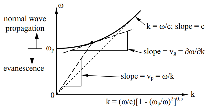
Using the expressions (9.5.19) and (9.5.20) for phase and group velocity we find for plasmas:

\[\mathrm{v}_{\mathrm{p}}=\omega / \mathrm{k}=\mathrm{c}\left[1-\left(\omega_{\mathrm{p}} / \omega\right)^{2}\right]^{-0.5}\]

\[\mathrm{v}_{\mathrm{g}}=(\partial \mathrm{k} / \partial \omega)^{-1}=\mathrm{c}\left[1-\left(\omega_{\mathrm{p}} / \omega\right)^{2}\right]^{0.5}\]

Since v_pv_g = c² , and since v_g ≤ c, it follows that v_p is always equal to or greater than c. However, for ω < ω_p we find v_p and v_g become imaginary because normal wave propagation is replaced by another behavior.

From (9.5.26) we see that when ω < ω_p:

\[\mathrm{\underline{k}=\frac{\omega}{c} \sqrt{1-\left(\omega_{p} / \omega\right)^{2}}=\pm j \alpha}\]

\[\underline{\eta}=\sqrt{\frac{\mu}{\varepsilon}}=\eta_{\mathrm{o}} / \sqrt{1-\left(\omega_{\mathrm{p}} / \omega\right)^{2}}=\mp \mathrm{j} \frac{\mu_{\mathrm{o}} \omega}{\alpha}\]

Therefore an x-polarized wave propagating in the +z direction would be:

\[\overline{\mathrm{\underline E}}=\hat{x} \mathrm{E}_{0} \mathrm{e}^{-\alpha \mathrm{z}}\]

\[\overline{\mathrm{H}}=\hat{y} \underline{\eta}^{-1} \underline{\mathrm{E}}_{\mathrm{o}} \mathrm{e}^{-\alpha z}=\mathrm{j} \hat{y}\left(\alpha / \omega \mu_{\mathrm{o}}\right) \mathrm{E}_{\mathrm{o}} \mathrm{e}^{-\alpha \mathrm{z}}\]

where the sign of ±jα was chosen (-) to correspond to exponential decay of the wave rather than growth. We find from (9.5.32) that H(t) is delayed 90^o behind E(t), that both decay exponentially with z, and that the Poynting vector \(\overline{\mathrm{\underline S}}\) is purely imaginary:

\[\overline{\mathrm{\underline S}}=\overline{\mathrm{\underline E}} \times \overline{\mathrm{\underline H}}^{*}=-\mathrm{j} \hat{z}\left(\alpha\left|\underline{\mathrm{E}}_{\mathrm{o}}\right|^{2} / \omega \mu_{\mathrm{o}}\right) \mathrm{e}^{-2 \alpha z}\]

Such an evanescent wave decays exponentially and carry only reactive power and no time-average power because of the time orthogonality of E and H. Reactive power implies that below ω_p the average energy stored is predominantly electric, but in this case the stored energy is actually dominated by the kinetic energy of the electrons. It is this extra energy that allows the permittivity ε to become negative below ω_p although μ_o remains constant. The frequency ω_p below which conversion from propagation to evanescence occurs is called the cut-off frequency, which is the plasma frequency here.

Example \(\PageIndex{C}\)

What is the plasma frequency f_p [Hz] of the ionosphere when n_e = 10¹² m^-3?

Solution

\(\mathrm{f}_{\mathrm{p}}=\omega_{\mathrm{p}} / 2 \pi=\left(10^{12} \mathrm{e}^{2} / \mathrm{m} \varepsilon_{0}\right)^{0.5} / 2 \pi \cong 9.0 \ \mathrm{MHz}\).