11.4: Applications

Wireless communications systems

Section 11.4.1 introduces simple communications systems without using Maxwell’s equations and Section 11.4.2 then discusses radar and lidar systems used for surveillance and research. Optical communications is deferred to Chapter 12, while the design, transformation, and switching of the communications signals themselves are issues left to other texts.

Wireless communications systems have a long history, beginning with wireless telegraph systems installed several years after Hertz’s laboratory demonstrations of wireless links late in the nineteenth century. These systems typically used line-of-sight propagation paths, and sometimes inter-continental ionospheric reflections. Telephone, radio, and television systems followed. In the mid-twentieth century, the longer interstate and international wireless links were almost entirely replaced by more capable and reliable coaxial cables and multi-hop microwave links. These were soon supplemented by satellite links typically operating at frequencies up to ~14 GHz; today frequencies up to ~100 GHz are used. At century’s end, these longer microwave links were then largely replaced again, this time by optical fibers with bandwidths of Terahertz. At the same time many of the shorter links are being replaced or supplemented by wireless cellular technology, which was made practical by the development of inexpensive r.f. integrated circuits. Each technical advance markedly boosted capacity and market penetration, and generally increased performance and user mobility while reducing costs.

Most U.S. homes and offices are currently served by twisted pairs of telephone wires, each capable of conveying ~50 kbs - 1.5 Mbps, although coaxial cables, satellite links, and wireless services are making significant inroads. The most common wireless services currently include cell phones, wireless phones (within a home or office), wireless internet connections, wireless intra-home and intra-office connections, walkie-talkies (dedicated mobile links), satellite links, microwave tower links, and many specialized variations designed for private or military use. In addition, optical or microwave line-of-sight links between buildings offer instant broadband connectivity for the “last mile” to some users; the last mile accounts for a significant fraction of all installed plant cost. Weather generally restricts optical links to very short hops or to weatherindependent optical fibers. Specialized wireless medical devices, such as RF links to video cameras inside swallowed pills, are also being developed.

Broadcast services now include AM radio near 1 MHz, FM radio near 100 MHz and higher frequencies, TV in several bands between 50 and 600 MHz for local over-the-air service, and TV and radio delivered by satellite at ~4, ~12, and ~20 GHz. Shortwave radio below ~30 MHz also offers global international broadcasts dependent upon ionospheric conditions, and is widely used by radio hams for long-distance communications.

Wireless services are so widespread today that we may take them for granted, forgetting that a few generations ago the very concept of communicating by invisible silent radio waves was considered magic. Despite the wide range of services already in use, it is reasonable to assume that over the next few decades numerous other wireless technologies and services will be developed by today’s engineering students.

Communications systems convey information between two or more nodes, usually via wires, wireless means, or optical fibers. After a brief discussion relating signaling rates (bits per second) to the signal power required at the wireless receiver, this section discusses in general terms the launching, propagation, and reception of electromagnetic signals and messages in wired and wireless systems.

Information is typically measured in bits. One bit of information is the information content of a single yes-no decision, where each outcome is equally likely. A string of M binary digits (equiprobable 0’s or 1’s) conveys M bits of information. An analog signal measured with an accuracy of one part in 2M also conveys M bits because a unique M-bit binary number corresponds to each discernable analog value. Thus both analog and digital signals can be characterized in terms of the bits of information they convey. All wireless receivers require that the energy received per bit exceed a rough minimum of w_o ≅ 10^-20 Joules/bit, although most practical systems are orders of magnitude less sensitive.⁵⁹

⁵⁹ Most good communications systems can operate with acceptable probabilities of error if E_b/N_o >~10, where E_b is the energy per bit and N_o = kT is the noise power density [W Hz^-1] = [J]. Boltzmann's constant k ≅ 1.38×10^-23 [J^o K^-1], and T is the system noise temperature, which might approximate 100K in a good system at RF frequencies. Thus the nominal minimum energy E_b required to detect each bit of information is ~10N_o ≅ 10^-20 [J].

To convey N bits per second [b s^-1] of information therefore requires that at least ~Nw_o watts [W] be intercepted by the receiver, and that substantially more power be transmitted. Note that [W] = [J s^-1] = [J b^-1][b s^-1]. Wireless communications is practical because so little power P_r is actually required at the receiver. For example, to communicate 100 megabits per second (Mbps) requires as little as one picowatt (10^-12 W) at the receiver if w_o = 10^-20; that is, we require P_r > Nw_o ≅ 10⁸ ×10^-20 = 10^-12 [W].

It is fortunate that radio receivers are so sensitive, because only a tiny fraction of the transmitted power usually reaches them. In most cases the path loss between transmitter and receiver is primarily geometric; the radiation travels in straight lines away from the transmitting antenna with an intensity I [W m^-2] that grows weaker with distance r as r^-2. For example, if the transmitter is isotropic and radiates its power P_t equally in all 4\(\pi\) directions, then I(θ,\(\phi\),r) = P_t/4\(\pi\)r² [W m^-2]. The power P_r intercepted by the receiving antenna is proportional to the incident wave intensity I(θ,\(\phi\)) and the receiving antenna effective area A(θ,\(\phi\)) [m²], or “capture cross-section”, where the power P_r received from a plane wave incident from direction θ,\(\phi\) is:

\[\mathrm{P}_{\mathrm{r}}=\mathrm{I}(\theta, \phi, \mathrm{r}) \mathrm{A}(\theta, \phi) \ [\mathrm{W}] \qquad \qquad \qquad \text{(antenna gain)} \label{11.4.1}\]

The power received from an isotropic transmitting antenna is therefore P_r = (P_t/4\(\pi\)r²)A(θ,\(\phi\)), so in this special case the line-of-sight path loss between transmitter and receiver is P_r/P_t = A(θ,\(\phi\))/4\(\pi\)r², or that fractional area of a sphere of radius r represented by the receiving antenna cross-section A. Sometimes additional propagation losses due to rain, gaseous absorption, or scattering must be recognized too, as discussed in Section 11.3.2.

In general, however, the transmitting antenna is not isotropic, but is designed to radiate power preferentially in the direction of the receivers. We define antenna gain G(θ,\(\phi\)), often called “gain over isotropic”, as the ratio of the intensity I(θ,\(\phi\),r) [W m^-2] of waves transmitted in the direction θ,\(\phi\) (spherical coordinates) at distance r, to the intensity that would be transmitted by an isotropic antenna. That is:

\[\mathrm{G}(\theta, \phi) \equiv \frac{\mathrm{I}(\theta, \phi, \mathrm{r})}{\mathrm{P}_{\mathrm{t}} / 4 \pi \mathrm{r}^{2}} \qquad \qquad \qquad \text{(antenna gain)} \label{11.4.2}\]

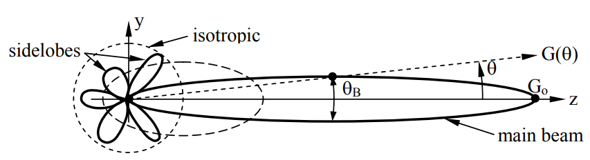
If the radiated power is conserved, then the integral of wave intensity over a spherical surface enclosing the antenna is independent of the sphere’s radius r. Therefore the angular distribution of power and G(θ,\(\phi\)) plotted in spherical coordinates behave much like a balloon that must push out somewhere when it is pushed inward somewhere else, as suggested in Figure 11.4.1. The maximum gain G_o often defines the z axis and is called the on-axis gain. The angular width θ_B of the main beam at the half-power points where G(θ,\(\phi\)) ≅ G_o/2 is called the antenna beamwidth or “half-power beamwidth”. Other local peaks in gain are called sidelobes, and those sidelobes behind the antenna are often called backlobes. Angles at which the gain is nearly zero are called nulls.

Figure \(\PageIndex{1}\): Isotropic and directive antenna gain patterns.

Antennas with G(θ,\(\phi\)) > 1 generally focus their radiated energy by using lenses, mirrors, or multiple radiators phased so their radiated contributions add in phase in the desired direction, and largely cancel otherwise. Typical gains for most wire antennas range from ~1.5 to ~100, and large aperture antennas such as parabolic dishes or optical systems can have gains of 10⁸ or more. The directionality or gain of a mirror or any antenna system is generally the same whether it is transmitting or receiving.⁶⁰ The fundamentals of transmission and reception are presented in more detail in Section 10.3.1.

⁶⁰ The degree of focus is the same whether the waves are transmitted or received. That is, if we reverse the direction of time for a valid electromagnetic wave solution to Maxwell’s equations, the result is also a valid solution if the system is lossless and reciprocal. Reciprocity requires that the complex matrices characterizing \(\underline{\varepsilon}\), \( \underline{\mu}\), and \( \underline{\sigma}\) near the antenna equal their own transposes; this excludes magnetized plasmas such as the ionosphere, and magnetized ferrites, as discussed further in Section 10.3.4.

Consider the following typical example. A television station transmits 100 kW at ~100 MHz toward the horizon with an antenna gain of ~10. Because the gain is much greater than unity in the desired horizontal direction, it is therefore less than unity for most other downward and upward directions where users are either nearby or absent. The intensity I [W m^-2] sensed by users on the horizon at 100-km range follows from (\ref{11.4.2}):

\[\mathrm{I} \cong \mathrm{G} \frac{\mathrm{P}_{\mathrm{t}}}{4 \pi \mathrm{r}^{2}}=10 \times \frac{10^{5}}{4 \pi\left(10^{5}\right)^{2}} \cong 10^{-5}\ \left[\mathrm{W} / \mathrm{m}^{2}\right]\label{11.4.3}\]

Whether this intensity is sufficient depends on the properties of the receiving antenna and receiver. For the example of Equation (\ref{11.4.3}), a typical TV antenna with an effective area A ≅ 2 [m²] would capture IA ≅ 10^-5[W/m²] × 2[m²] = 2×10^-5 [W]. If the received power is \(\left\langle\mathrm{v}^{2}(\mathrm{t})\right\rangle / \mathrm{R} \cong 2 \times 10^{-5} \ [\mathrm{W}] \), and the receiver has an input impedance R of 100 ohms, then the rootmean-square (rms) voltage \(\mathrm{v}_{\mathrm{rms}} \equiv\left\langle\mathrm{v}^{2}(\mathrm{t})\right\rangle^{0.5} \) would be (0.002)^0.5 ≅ 14 mv, much larger than typical noise levels in TV receivers (~10 μv).⁶¹

⁶¹ Typical TV receivers might have a superimposed noise voltage of power N = kTB [W], where the system noise temperature T might be ~10⁴ K (much is interference), Boltzmann's constant k = 1.38×10^-23, and B is bandwidth [Hz]. B ≅ 6 MHz for over-the-air television. Therefore N ≅ 1.38×10^-23×10⁴×6×10⁶ ≅ 8×10^-13 watts, and a good TV signal-to-noise ratio S/N of ~10⁴ requires only ~ 8×10^-9 watts of signal S. Since N ≅ n_rms² /R, the rms noise voltage ≅ (NR)^0.5, or ~10 μv if the receiver input impedance R = 100 ohms.

Because most antennas are equally focused whether they are receiving or transmitting, their effective area A(θ,\(\phi\)) and gain G(θ,\(\phi\)) are closely related:

\[\mathrm{G}(\theta, \phi)=\frac{4 \pi}{\lambda^{2}} \mathrm{A}(\theta, \phi) \label{11.4.4}\]

Therefore the on-axis gain \( \mathrm{G}_{\mathrm{o}}=4 \pi \mathrm{A}_{\mathrm{o}} / \lambda^{2}\). This relation (\ref{11.4.4}) was proven for a short dipole antenna in Section 10.3.3 and proven for other types of antenna in Section 10.3.4, although the proof is not necessary here. This relation is often useful in estimating the peak gain of aperture antennas like parabolic mirrors or lenses because their peak effective area A_o often approaches their physical cross-section A_p within a factor of two; typically A_o ≅ 0.6 A_p. This approximation does not apply to wire antennas, however. Thus we can easily estimate the on-axis gain of such aperture antennas:

\[\mathrm{G}_{\mathrm{o}}=0.6 \times \frac{4 \pi}{\lambda^{2}} \mathrm{A}_{\mathrm{o}} \label{11.4.5}\]

Combining (\ref{11.4.1}) and (\ref{11.4.3}) yields the link expression for received power:

\[\mathrm{P}_{\mathrm{r}}=\mathrm{G}_{\mathrm{t}} \frac{\mathrm{P}_{\mathrm{t}}}{4 \pi \mathrm{r}^{2}} \mathrm{A}_{\mathrm{r}} \ [\mathrm{W}] \qquad \qquad \qquad \text{(link expression) } \label{11.4.6}\]

where G_t is the gain of the transmitting antenna and A_r is the effective area of the receiving antenna. The data rate R associated with this received power is : R = P_r/E_b [bits s^-1].

A second example illustrates how a communications system might work. Consider a geosynchronous communications satellite⁶² transmitting 12-GHz high-definition television (HDTV) signals at 20 Mbps to homes with 1-meter dishes, and assume the satellite antenna spreads its power P_t roughly equally over the eastern United States, say 3×10⁶ km² . Then the intensity of the waves falling on the U.S. is: I ≅ P_t/(3×10¹²) [W m^-2], and the power P_r received by an antenna with effective area A_o ≅ 0.6 [m²] is:

\[\mathrm{P}_{\mathrm{r}}=\mathrm{A}_{\mathrm{o}} \mathrm{I}=0.6 \frac{\mathrm{P}_{\mathrm{t}}}{3 \times 10^{12}}=2 \times 10^{-13} \mathrm{P}_{\mathrm{t}} \ [\mathrm{W}] \label{11.4.7}\]

⁶² A satellite approximately 35,000 km above the equator circles the earth in 24 hours at the same rate at which the earth rotates, and therefore can remain effectively stationary in the sky as a communications terminal serving continental areas. Such satellites are called “geostationary” or “geosynchronous”.

If E_b = 10^-20 Joules per bit suffices, then an R = 20-Mbps HDTV signal requires:

\[\mathrm{P}_{\mathrm{r}}=\mathrm{E}_{\mathrm{b}} \mathrm{R}=10^{-20} \times\left(2 \times 10^{7}\right)=2 \times 10^{-13} \ [\mathrm{W}] \label{11.4.8}\]

The equality of the right-hand parts of (\ref{11.4.7}) and (\ref{11.4.8}) reveals that one watt of transmitter power P_t in this satellite could send a digital HDTV signal to all the homes and businesses in the eastern U.S. Since a 20-dB margin⁶³ for rain attenuation, noisy receivers, smaller or poorly pointed home antennas, etc. is desirable, 100-watt transmitters might be used in practice.

⁶³ Decibels (dB) are defined for a ratio R such that dB = 10 log₁₀R and R = 10^(dB)/10; thus 20 dB → R = 100.

We can also estimate the physical area A_p of the aperture antenna on the satellite. If we know P_t and I at the earth, then we can determine the satellite gain G using I = GP_t/4\(\pi\)r² (\ref{11.4.2}), where r ≅ 40,000 km in the northern U.S; here we have I ≅ 3.3×10^-12 when P_t = 1 watt. The wavelength λ at 12 GHz is 2.5 cm (λ = c/f). But A_p ≅ 1.5A_o, where A_o is related to G by (\ref{11.4.4}). Therefore we obtain the reasonable result that a 2.5-meter diameter parabolic dish on the satellite should suffice:

\[\mathrm{A_{p} \cong 1.5 A_{0}=\left(1.5 \lambda^{2} / 4 \pi\right) G=\left(1.5 \lambda^{2} / 4 \pi\right)\left(4 \pi r^{2} I / P_{t}\right) \cong 5 \ \left[m^{2}\right]} \label{11.4.9}\]

The same result could have been obtained by determining the angular extent of the U.S. coverage area as seen from the satellite and then, as discussed in Section 11.1.2, determining what diameter antenna would have a diffraction pattern with that same beamwidth.

Thus we can design digital communications systems for a data rate R [b s^-1] if we know the range r, wavelength λ, and receiver sensitivity (Joules required per bit). For analog systems we also need to know the desired signal-to-noise ratio (SNR) at the receiver and the noise power N. Table 11.4.1 lists typical data rates R for various applications, and Table 11.4.2 lists typical SNR values required for various types of analog signal.

Table \(\PageIndex{1}\): Digital data rates for typical applications and source coding techniques⁶⁴.

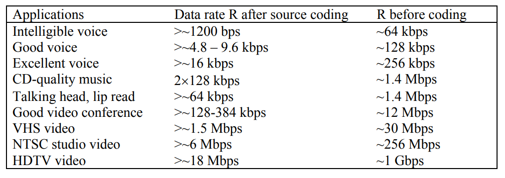
⁶⁴ Source coding reduces the number of bits to be communicated by removing redundancies and information not needed by the user. The table lists typical data rates before and after coding.

Table \(\PageIndex{2}\): Signal-to-noise ratios⁶⁵ for typical wireless applications.

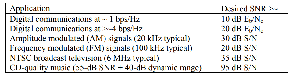
⁶⁵ For digital signals the dimensionless signal-to-noise ratio (SNR) given here is the energy-per-bit E_b divided by the noise power density N_o [W Hz^-1], where N_o = kT and T is the noise temperature, say 100-10⁴ K typically. For analog signals, S and N are the total signal and noise powers, respectively, where N = kTB and B is signal bandwidth [Hz].

Example \(\PageIndex{A}\)

A parabolic reflector antenna of 2-meter diameter transmits P_t = 10 watts at 3 GHz from beyond the edge of the solar system (R ≅ 10¹⁰ km) to a similar antenna on earth of 50-m diameter at a maximum data rate N bits/sec. What is N if the receiver requires 10^-20 Joules bit^-1?

Solution

Recall that the on-axis effective area A of a circular aperture antenna equals ~0.6 times its physical area (\(\pi\)r²), and it has gain \(\mathrm{G}=4 \pi \mathrm{A} / \lambda^{2}=(2 \pi \mathrm{r} / \lambda)^{2}\). The received power is \(\mathrm P_{\mathrm{rec}}=\mathrm{P}_{\mathrm{t}} \mathrm{G}_{\mathrm{t}} \mathrm{A}_{\mathrm{r}} / 4 \pi \mathrm{R}^{2} \) (\ref{11.4.6}); therefore:

\[\begin{aligned}\mathrm{R} \cong \mathrm{P}_{\mathrm{rec}} / \mathrm{E}_{\mathrm{b}} &=\left[\mathrm{P}_{\mathrm{t}}(0.6)^{2}\left(2 \pi \mathrm{r}_{\mathrm{t}} / \lambda\right)^{2} \pi \mathrm{r}_{\mathrm{r}}^{2}\right] /\left[4 \pi \mathrm{R}^{2} \mathrm{E}_{\mathrm{b}}\right] \\ &=\left[10 \times(0.6)^{2}(2 \pi \times 1 / 0.1)^{2} \pi 25^{2}\right] /\left[4 \pi 10^{26} \times 10^{-20}\right] \cong 2.2 \ \mathrm{bps} \end{aligned}\]

Radar and lidar

Radar (RAdio Direction and Range finding) and lidar (LIght Direction and Range finding) systems transmit signals toward targets of interest and receive echoes. They typically determine: 1) target distance using the round-trip propagation delay, 2) target direction using echo strength relative to antenna orientation, 3) target radial velocity using the observed Doppler shift, and 4) target size or scattering properties using the maximum echo strength. Figure 11.4.2 illustrates the most common radar configuration.

Figure \(\PageIndex{2}\): Radar signals reflected from a target.

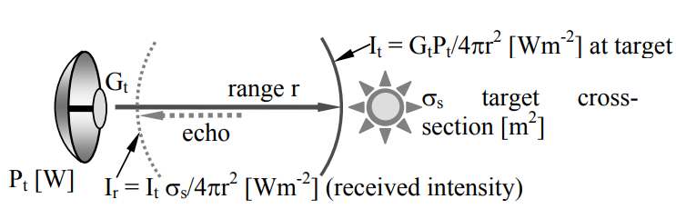
To compute the received power, we first compute the intensity I_t of radiation at the target at range r for a transmitter power and antenna gain of P_t and G, respectively:

\[\mathrm{I}_{\mathrm{t}}=\mathrm{G} \frac{\mathrm{P}_{\mathrm{t}}}{4 \pi \mathrm{r}^{2}} \ \left[\mathrm{W} / \mathrm{m}^{2}\right] \qquad \qquad \qquad \text{(intensity at target) } \label{11.4.10}\]

The target then scatters this radiation in some pattern and absorbs the rest. Some of this scattered radiation reaches the receiver with intensity I_r, where:

\[\mathrm{I}_{\mathrm{r}}=\mathrm{I}_{\mathrm{t}} \frac{\sigma_{\mathrm{s}}}{4 \pi \mathrm{r}^{2}} \ \left[\mathrm{W} / \mathrm{m}^{2}\right] \qquad \qquad \qquad \text{(intensity at radar) } \label{11.4.11}\]

where \(\sigma_{\mathrm{s}} \) is the scattering cross-section of the target and is defined by (\ref{11.4.11}). That is, \(\sigma_{\mathrm{s}} \) is the capture cross-section [m²] at the target that would produce I_r if the target scattered incident radiation isotropically. Thus targets that preferentially scatter radiation toward the transmitter can have scattering cross-sections substantially larger than their physical cross-sections.

The received power P_r is then simply I_rA_r [W], where A_r is the effective area of the receiving antenna. That is:

\[\mathrm{P_{r}=I_{r} A_{r}=\frac{I_{t} \sigma_{s}}{4 \pi r^{2}} A_{r}=G \frac{P_{t} \sigma_{s}}{\left(4 \pi r^{2}\right)^{2}} A_{r}} \label{11.4.12}\]

\[\mathrm{P_{r}=P_{t} \frac{\sigma_{s}}{4 \pi}\left(\frac{G \lambda}{4 \pi r^{2}}\right)^{2} \ [W]} \qquad\qquad\qquad \text{(radar equation)} \label{11.4.13}\]

where we used \( \mathrm{A}_{\mathrm{r}}=\mathrm{G} \lambda^{2} / 4 \pi\), and where (\ref{11.4.13}) is often called the radar equation. The dependence of received power on the fourth power of range and the square of antenna gain often control radar system design.

Atmospheric attenuation is often included in the radar equation by means of a round-trip attenuation factor \( \mathrm{e^{-2 \alpha r}}\), where \(\alpha\) is the average atmospheric attenuation coefficient (m^-1) and r is range. Atmospheric attenuation is discussed in Section 11.3.2 and below 200 GHz is due principally to oxygen, water vapor, and rain; it is usually not important below ~3 GHz. Oxygen absorption occurs primarily in the lowest 10 km of the atmosphere ~50-70 GHz and near 118 GHz, water vapor absorption occurs primarily in the lowest 3 km of the atmosphere above ~10 GHz, and rain absorption occurs up to ~15 km in the largest rain cells above ~3 GHz.

Lidar systems also obey the radar equation, but aerosol scattering by clouds, haze, or smoke becomes more of a concern. Also the phase fronts of optical beams are more easily disturbed by refractive inhomogeneities in the atmosphere that can modulate received echoes on time scales of milliseconds with random fading of ten dB or more.

A simple example illustrates use of the radar equation (\ref{11.4.13}). Suppose we wish to know the range r at which we can detect dangerous asteroids having diameters over ~300m that are approaching the earth. Assume the receiver has additive noise characterized by the system noise temperature T_s, and that the radar bandwidth is one Hertz because the received sinusoid will be averaged for approximately one second. Detectable radar echos must have P_r > kT_sB [W], where k is Boltzmann's constant (k = 1.38×10^-23) and B is the system bandwidth (~1 Hz); this implies P_r ≅ 1.4×10^-23 T_s watts. We can estimate \( \sigma_{\mathrm{s}}\) for a 300-meter asteroid by assuming it reflects roughly as well as the earth, say fifteen percent, and that the scattering is roughly isotropic; then \(\sigma_{\mathrm{s}} \cong 10^{4} \) [m²]. If we further assume our radar is using near state-of-the-art components, then we might have P_t ≅ 1 Mw, Gt ≅ 10⁸, λ = 0.1 m, and T_s ≅ 10K. The radar equation then yields:

\[\mathrm{r} \cong\left[\mathrm{P}_{\mathrm{t}} \sigma_{\mathrm{s}}\left(\mathrm{G}_{\mathrm{t}} \lambda\right)^{2} /(4 \pi)^{3} \mathrm{P}_{\mathrm{r}}\right]^{0.25} \cong 5 \times 10^{7} \ \mathrm{km} \label{11.4.14}\]

This range is about one-third of the distance to the sun and would provide about 2-3 weeks warning.

Optical systems with a large aperture area A might perform this task better because their antenna gain \(\mathrm{G}=\mathrm{A} 4 \pi / \lambda^{2} \), and λ for lidar is typically 10^-5 that of a common radar. For antennas of the same physical aperture and transmitter power, 1-micron lidar has an advantage over 10-cm radar of ~10¹⁰ in P_r/P_t.

Radar suffers because of its dependence on the fourth power of range for targets smaller than the antenna beamwidth. If the radar can place all of its transmitted energy on target, then it suffers only the range-squared loss of the return path. The ability of lidar systems to strongly focus their transmitting beam totally onto a small target often enables their operation in the highly advantageous r^-2 regime rather than r^-4.

Equations (\ref{11.4.13}) and (\ref{11.4.14}) can easily be revised for the case where all the radar energy intercepts the target. The radar equation then becomes:

\[\mathrm{P_{r}=P_{t} R G(\lambda / 4 \pi r)^{2} \ [W]} \label{11.4.15}\]

where the target retro-reflectivity R is defined by (\ref{11.4.15}) and is the dimensionless ratio of back-scattered radiation intensity at the radar to what would be back scattered if the radiation were scattered isotropically by the target. For the same assumptions used before, asteroids could be detected at a range r of ~3×10¹² km if R ≅ 0.2, a typical value for icy rock. The implied detection distance is now dramatically farther than before, and reaches outside our solar system. However, the requirement that the entire radar beam hit the asteroid would be essentially impossible even for the very best optical systems, so this approach to boosting detection range is usually not practical for probing small distant objects.

Radar systems often use phased arrays of antenna elements, as discussed in Section 10.4, to focus their energy on small spots or to look in more than one direction at once. In fact a single moving radar system, on an airplane for example, can coherently receive sequential reflected radar pulses and digitally reassemble the signal over some time period so as to synthesize the equivalent of a phased array antenna that is far larger than the physical antenna. That is, a small receiving antenna can be moved over a much larger area A, and by combining its received signals from different locations in a phase-coherent way, can provide the superior angular resolution associated with area A. This is called synthetic aperture radar (SAR) and is not discussed further here.

Example \(\PageIndex{B}\)

A radar with 1-GHz bandwidth and 40-dB gain at 10 GHz views the sun, which has angular diameter 0.5 degrees and brightness temperature T_B = 10,000K. Roughly what is the antenna temperature T_A and the power received by the radar from the sun if we ignore any radar reflections?

Solution

The power received is the intensity at the antenna port I [W/Hz] times the bandwidth B [Hz], where I ≅ kT_A (11.3.1), and T_A is the antenna temperature given by the integral in (11.3.4). This integral is trivial if G(θ,\(\phi\)) is nearly constant over the solid angle \(\Omega_{\mathrm{S}}\) of the sun; then \( \mathrm{T}_{\mathrm{A}} \cong \mathrm{G}_{\mathrm{o}} \mathrm{T}_{\mathrm{B}} \Omega_{\mathrm{S}} / 4 \pi\). Constant gain across the sun requires the antenna beamwidth θ_B >> 0.5 degrees. We can roughly estimate θ_B by approximating the antenna gain as a constant G_o over solid angle \(\Omega_{\mathrm{B}}\), and zero elsewhere; then (10.3.3) yields \(\int_{4 \pi} \mathrm{G}(\theta, \phi) \mathrm{d} \Omega=4 \pi=\mathrm{G}_{0} \Omega_{\mathrm{B}}=10^{4} \Omega_{\mathrm{B}} \). Therefore \( \Omega_{\mathrm{B}} \cong 4 \pi / 10^{4} \cong \pi\left(\theta_{\mathrm{B}} / 2\right)^{2}\), and θ_B ≅ 0.04 radians ≅ 2.3 degrees, which is marginally greater than the solar diameter required for use of the approximation θ_B >> 0.5 in a rough estimate. It follows that \(\mathrm{T}_{\mathrm{A}} \cong \mathrm{G}_{\mathrm{o}} \mathrm{T}_{\mathrm{B}} \Omega_{\mathrm{S}} / 4 \pi=10^{4} \times 10^{4} \times \pi\left(\theta_{\mathrm{S}} / 2\right)^{2} / 4 \pi \cong 480 \) degrees Kelvin, somewhat larger than the noise temperature of good receivers. The power received is \(\mathrm{kT}_{\mathrm{A}} \mathrm{B} \cong 1.38 \times 10^{-23} \times 480 \times 10^{9} \cong 6.6 \times 10^{-12} \ \mathrm{watts} \). This is a slight overestimate because the gain is actually slightly less than G_o at the solar limb.

Example \(\PageIndex{C}\)

What is the scattering cross-section \(\sigma_{\mathrm{s}}\) of a small distant flat plate of area F oriented so as to reflect incident radiation directly back toward the transmitter?

Solution

The radar equation (\ref{11.4.12}) relates the transmitted power P_t to that received, P_r, in terms of \(\sigma_{\mathrm{s}}\). A similar relation can be derived by treating the power reflected from the flat plate as though it came from an aperture uniformly illuminated with intensity P_tG_t/4\(\pi\)r² [W m^-2]. The power P_r received by the radar is then the power radiated by the flat-plate aperture, FP_tG_t/4\(\pi\)r² [W], inserted as P_t into the link expression (\ref{11.4.6}): P_r = (FP_tG_t/4\(\pi\)r²)G_fA_r/4\(\pi\)r² . The gain of the flat plate aperture is \( \mathrm{G}_{\mathrm{f}}=\mathrm{F} 4 \pi / \lambda^{2}\), and \( \mathrm{A}_{\mathrm{r}}=\mathrm{G} \lambda^{2} / 4 \pi\), so G_fA_r = GF. Equating P_r in this expression to that in the radar equation yields: \(\mathrm{P}_{\mathrm{t}} \sigma_{\mathrm{s}}\left(\mathrm{G} \lambda / 4 \pi \mathrm{r}^{2}\right)^{2} / 4 \pi=\left(\mathrm{FP}_{\mathrm{t}} \mathrm{G}_{\mathrm{t}} / 4 \pi \mathrm{r}^{2}\right) \mathrm{GF} / 4 \pi \mathrm{r}^{2} \), so \( \sigma_{\mathrm{s}}=\mathrm{F}\left(4 \pi \mathrm{F} / \lambda^{2}\right)\). Note \(\sigma_{\mathrm{s}}\) >> F if \( \mathrm{F}>>\lambda^{2} / 4 \pi\). Corner reflectors (three flat plates at right angles intersecting so as to form one corner of a cube) reflect plane waves directly back toward their source if the waves impact the concave portion of the reflector from any angle. Therefore the corner reflector becomes a very area-efficient radar target if its total projected area F is larger than \( \lambda^{2}\).