7.3: Methods for Matching Transmission Lines

Frequency-Dependent Behavior

This section focuses on the frequency-dependent behavior introduced by obstacles and impedance transitions in transmission lines, including TEM lines, waveguides, and optical systems. Frequency-dependent transmission line behavior can also be introduced by loss, as discussed in Section 8.3.1, and by the frequency-dependent propagation velocity of waveguides and optical fibers, as discussed in Sections 9.3 and 12.2.

The basic issue is illustrated in Figure 7.3.1(a), where an obstacle reflects some fraction of the incident power. If we wish to eliminate losses due to reflections we need to cancel the reflected wave by adding another that has the same magnitude but is 180° out of phase. This can easily be done by adding another obstacle in front of or behind the first with the necessary properties, as suggested in (b). However, the reflections from the further obstacle can bounce between the two obstacles multiple times, and the final result must consider these additional rays too. If the reflections are small the multiple reflections become negligible. This strategy works for any type of transmission line, including TEM lines, waveguides and optical systems.

Figure \(\PageIndex{1}\): Cancellation of reflections on transmission lines.

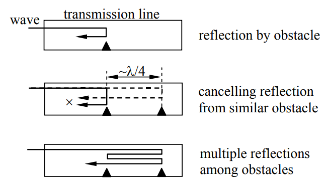
The most important consequence of any such tuning strategy to eliminate reflections is that the two reflective sources are often offset spatially, so the relative phase between them is wavelength dependent. If multiple reflections are important, this frequency dependence can increase substantially. Rather than consider all these reflections in a tedious way, we can more directly solve the equations by extending the analysis of Section 7.2.3, which is summarized below in the context of TEM lines having characteristic admittance Y_o and a termination of complex impedance \(\underline{\mathrm{Z}}_{\mathrm{L}}\):

\[\underline{V}(\mathrm{z})=\underline{\mathrm{V}}_{+} \mathrm{e}^{-\mathrm{jkz}}+\underline{\mathrm{V}}_{-} \mathrm{e}^{\mathrm{jkz}}\ [\mathrm{V}]\]

\[\underline{I}(\mathrm z)=Y_{0}\left(\underline{V}_{+} e^{-j k z}-\underline{V}_{-} e^{j k z}\right) \ [A]\]

\[\underline{\Gamma}(\mathrm{z}) \equiv\left(\underline{\mathrm{V}}_{-} \mathrm{e}^{\mathrm{jkz}}\right) /\left(\underline{\mathrm{V}}_{+} \mathrm{e}^{-\mathrm{jkz}}\right)=\left(\underline{\mathrm{V}}-\underline{\mathrm{V}}_{+}\right) \mathrm{e}^{2 \mathrm{jkz}}=\left(\underline{\mathrm{Z}}_{\mathrm{n}}-1\right) /\left(\underline{\mathrm{Z}}_{\mathrm{n}}+1\right)\]

The normalized impedance \(\underline{Z}_{\mathrm n}\) is defined as:

\[\underline{Z}_{\mathrm n} \equiv \underline{Z} / Z_{o}=[1+\underline{\Gamma}(z)] /[1-\underline{\Gamma}(z)]\]

\( \underline{Z}_{\mathrm n}\) can be related to \( \underline{\Gamma}(\mathrm{z})\) by dividing (7.3.1) by (7.3.2) to find \(\underline{\mathrm{Z}}(\mathrm{z}) \), and the inverse relation (7.3.3) follows. Using (7.3.3) and (7.3.4) in the following sequences, the impedance \(\underline{Z}\left(\mathrm{z}_{2}\right)\) at any point on an unobstructed line can be related to the impedance at any other point z₁:

\[\underline{Z}\left(z_{1}\right) \Leftrightarrow \underline{Z}_{n}\left(z_{1}\right) \Leftrightarrow \underline{\Gamma}\left(z_{1}\right) \Leftrightarrow \underline{\Gamma}\left(z_{2}\right) \Leftrightarrow \underline{Z}_{n}\left(z_{2}\right) \Leftrightarrow \underline{Z}\left(z_{2}\right)\]

The five arrows in (7.3.5) correspond to application of equations (7.3.3) and (7.3.4) in the following left-to-right sequence: (4), (3), (3), (4), (4), respectively.

One standard problem involves determining \(\underline{Z}(\mathrm{z})\) (for z < 0) resulting from a load impedance \(\underline{\mathrm{Z}}_{\mathrm{L}}\) at z = 0. One approach is to replace the operations in (7.3.5) by a single equation, derived in (7.2.24):

\[\underline{Z}(\mathrm{z})=\mathrm{Z}_{0}\left(\underline{\mathrm{Z}}_{\mathrm{L}}-\mathrm{j} \mathrm{Z}_{\mathrm{o}} \tan \mathrm{kz}\right) /\left(\mathrm{Z}_{\mathrm{o}}-\mathrm{j} \underline{\mathrm{Z}}_{\mathrm{L}} \text { tan } \mathrm{kz}\right) \qquad\qquad\qquad \text { (impedance transformation) }\]

For example, if \(\underline{\mathrm{Z}}_{\mathrm{L}}=0\), then \(\underline{\mathrm{Z}}(\mathrm{z})=-\mathrm{j} \mathrm{Z}_{\mathrm{o}} \tan \mathrm{kz}\), which means that \(\underline{Z}(z)\) can range between -j∞ and +j∞, depending on z, mimicking any reactance at a single frequency. The impedance repeats at distances of Δz = λ, where k(Δz) = (2π/λ)Δz = 2π. If \(\underline{Z}_{L}=Z_{0}\), then \(\underline{Z}(z)=Z_{0}\) everywhere.

Example \(\PageIndex{A}\)

What is the impedance at 100 MHz of a 100-ohm TEM line λ/4 long and connected to a: 1) short circuit? 2) open circuit? 3) 50-ohm resistor? 4) capacitor C = 10^-10 F?

Solution

In all four cases the relation between \(\underline{\Gamma}(z=0)=\underline{\Gamma}_{L}\) at the load, and \(\underline{\Gamma}(z=-\lambda / 4)\) is the same [see (7.3.3)]:

\[\underline{\Gamma}(z=-\lambda / 4)=\underline{\Gamma}_{\underline{L}} \mathrm{e}^{2 \overline{\mathrm{j}} \mathrm{k} z}=\underline{\Gamma}_{\underline{L}} \mathrm{e}^{2 \mathrm{j}(2 \pi / \lambda)(-\lambda / 4)}=-\underline{\Gamma}_{\underline{L}}.\nonumber\]

Therefore in all four cases we see from (7.3.4) that

\[\underline{Z}_{n}(\mathrm{z}=-\lambda / 4)=\left(1-\underline{\Gamma}_{\mathrm{L}}\right) /\left(1+\underline{\Gamma}_{\mathrm{\underline{L}}}\right)=1 / \underline{\mathrm{Z}}_{\mathrm{n}}(0) \cdot \underline{\mathrm{Z}}_{\mathrm{n}}(\mathrm{z}=0)\nonumber\]

for these four cases is: 0, ∞, 0.5, and \(1 / j \omega C Z_{0}=1 /\left(j 2 \pi 10^{8} 10^{-10} 100\right)=1 / j 2 \pi\), respectively. Therefore \(\underline{Z}(z=-\lambda / 4)=100 \underline{Z}_{\mathrm{n}}^{-1} \text {ohms }\), respectively. Since the impedance of an inductor is \(\underline{Z}=j \omega L\), it follows that j200π is equivalent at 100 MHz to \(\mathrm{L}= 200 \pi / \omega=200 \pi / 200 \pi 10^{8}=10^{-8} \ [\mathrm{Hy}]\).

Smith chart, stub tuning, and quarter-wave transformers

A common problem is how to cancel reflections losslessly, thus forcing all incident power into a load. This requires addition of one or more reactive impedances in series or in parallel with the line so as to convert the impedance at that point to Z_o, where it must remain for all points closer to the source or next obstacle. Software tools to facilitate this have been developed, but a simple graphical tool, the Smith chart, provides useful insight into what can easily be matched and what cannot. Prior to computers it was widely used to design and characterize microwave systems.

The key operations in (7.3.5) are rotation on the gamma plane \(\left[\underline{\Gamma}\left(z_{1}\right) \Leftrightarrow \underline{\Gamma}\left(z_{2}\right)\right]\) and the conversions \(\underline{Z}_{n} \Leftrightarrow \underline{\Gamma}\), given by (7.3.3–4). Both of these operations can be accommodated on a single graph that maps the one-to-one relationship \(\underline{Z}_{n} \Leftrightarrow \underline{\Gamma}\) on the complex gamma plane, as suggested in Figure 7.3.2(a). Conversions \(\underline{\Gamma}\left(z_{1}\right) \Leftrightarrow \underline{\Gamma}\left(z_{2}\right)\) are simply rotations on the gamma plane. The gamma plane was introduced in Figure 7.2.3. The Smith chart simply overlays the equivalent normalized impedance values \(\underline{\mathrm{Z}}_{\mathrm{n}}\) on the gamma plane; only a few key values are indicated in the simplified version shown in (a). For example, the loci for which the real R_n and imaginary parts X_n of \(\underline{\mathrm{Z}}_{\mathrm{n}}\) remain constant lie on segments of circles \(\left(\underline{Z}_{n} \equiv R_{n}+j X_{n}\right)\).

Figure \(\PageIndex{2}\): Relation between the gamma plane and the Smith chart.

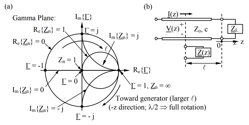
Rotation on the gamma plane relates the values of \(\underline{\mathrm{Z}}_{\mathrm{n}}\) and \(\underline{\Gamma}\) at one z to their values at another, as suggested in Figure 7.3.2(b). Since \(\underline{\Gamma}(\mathrm{z})=\left(\underline{\mathrm{V}}_{-}/\underline{\mathrm{V}}_{+}\right) \mathrm{e}^{2 \mathrm{jkz}}=\underline{\Gamma}_{\mathrm{L}} \mathrm{e}^{2 \mathrm{jkz}}=\underline{\Gamma}_{\mathrm{L}} \mathrm{e}^{-2 \mathrm{jk} \ell}\), and since e^jφ corresponds to counter-clockwise rotation as φ increases, movement toward the generator (-z direction) corresponds to clockwise rotation in the gamma plane. The exponent of \(\mathrm{e}^{-2 \mathrm{jk} \ell}\) is ­\(-\mathrm{j} 4 \pi \ell / \lambda\), so a full rotation on the gamma plane corresponds to movement \(\ell\) down the line of only λ/2.

A simple example illustrates the use of the Smith chart. Consider an inductor having jωL = j100 on a 100-ohm line. Then \(\underline{Z}_{n}=j \), which corresponds to a point at the top of the Smith chart where \(\underline{\Gamma}=+j \) (normally \(\left.\underline{Z}_{n} \neq \underline{\Gamma}\right)\). If we move toward the generator λ/4, corresponding to rotation of \(\underline{\Gamma}(\mathrm{z}) \) half way round the Smith chart, then we arrive at the bottom where \( \underline{\mathrm{Z}}_{\mathrm{n}}=-\mathrm{j}\) and \(\underline{Z}=Z_{0} \underline{Z}_{n}=-\mathrm{j} 100=1 / \mathrm{j} \omega \mathrm{C}\). So the equivalent capacitance C at the new location is 1/100ω farads.

The Smith chart has several other interesting properties. For example, rotation half way round the chart (changing \(\underline{\Gamma}\) and \(-\underline{\Gamma}\)) converts any normalized impedance into the corresponding normalized admittance. This is easily proved: since \(\underline{\Gamma}=\left(\underline{Z}_{n}-1\right) /\left(\underline{Z}_{n}+1\right)\), conversion of \(\underline{Z}_{n} \rightarrow \underline{\mathrm{Z}}_{\mathrm{n}}^{-1}\) yields \(\underline{\Gamma}^{\prime}=\left(\underline{Z}_{\mathrm{n}}^{-1}-1\right) /\left(\underline{\mathrm{Z}}_{\mathrm{n}}^{-1}+1\right)=\left(1-\mathrm{Z}_{\mathrm{n}}\right) /\left(\mathrm{Z}_{\mathrm{n}}+1\right)=-\underline{\Gamma} \ [\mathrm{Q} . \mathrm{E} . \mathrm{D} .]^{35}\) Pairs of points with this property include \( \underline{\mathrm{Z}}_{\mathrm{n}}=\pm \mathrm{j}\) ad \(\underline{\mathrm{Z}}_{\mathrm{n}}=(0, \infty)\).

³⁵ Q.E.D. is an abbreviation for the Latin phrase “quod erat demonstratum”, or “that which was to be demonstrated”.

Another useful property of the Smith chart is that the voltage-standing-wave ratio (VSWR) equals the maximum positive real value R_{n max} of \(\underline{\mathrm{Z}}_{\mathrm{n}} \) lying on the circular locus occupied by \(\underline{\Gamma}(\mathrm{z}) \). This is easily shown from the definition of VSWR:

\[\begin{align}
\mathrm{VSWR} & \equiv|\underline{\mathrm{V}} \max |\left|\mathrm{V}_{\min }\right|=\left(\left|\mathrm{V}_{+} \mathrm{e}^{-\mathrm{j} \mathrm{kz}}\right|+\left|\mathrm{V}_{-} \mathrm{e}^{+\mathrm{jkz}}\right|\right) /\left(\left|\mathrm{V}_{+} \mathrm{e}^{-\mathrm{jkz}}\right|-\left|\mathrm{V}_{-} \mathrm{e}^{+\mathrm{jkz}}\right|\right) \nonumber \\
& \equiv(1+|\underline{\mathrm{I}}|) /(1-|\underline{\mathrm{I}}|)=\mathrm{R}_{\mathrm{n} \max }
\end{align}\]

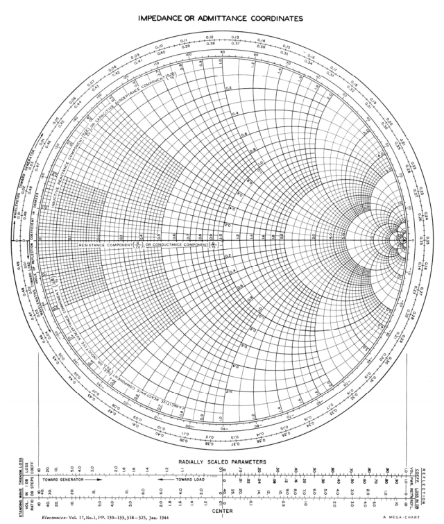
A more important use of the Smith chart is illustrated in Figure 7.3.3, where the load 60 + j80 is to be matched to a 100-ohm TEM line so all the power is dissipated in the 60-ohm resistor. In particular the length \( \ell\) of the transmission line in Figure 7.3.3(a) is to be chosen so as to transform \( \underline{Z}_{L}=60+80 j\) so that its real part becomes Z_o. The new imaginary part can be canceled by a reactive load (L or C) that will be placed either in position M or N. The first step is to locate \(\underline{\mathrm{Z}}_{\mathrm{n}} \) on the Smith chart at the intersection of the R_n = 0.6 and X_n = 0.8 circles, which happen to fall at \(\underline{\Gamma} \). Next we locate the gamma circle \( \underline{\Gamma}(\mathrm{z})\) along which we can move by varying \( \ell\). This intersects the R_n = 1 circle at point “a” after rotating toward the generator “distance A”. Next we can add a negative reactance to cancel the reactance jX_n = +1.18j at point “a” to yield \(\underline{Z}_{n}(a)=1\) and \(\underline{Z}=Z_{0}\). A negative reactance is a capacitor C in series at location M in the circuit. Therefore 1/jωC = -1.18jZ_o and C = (1.18ωZ_o)^-1. The required line length \(\ell\) corresponds to ~0.05λ, a scale for which is printed on the perimeter of official charts as illustrated in Figure 7.3.4.

Figure \(\PageIndex{3}\): Matching a reactive load using the Smith chart.

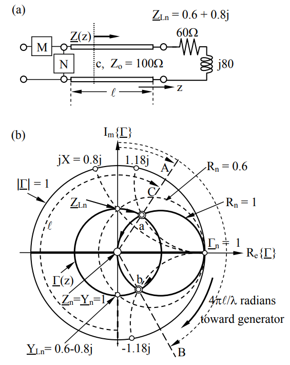
More than three other matching schemes can be used here. For example, we could lengthen \( \ell\) to distance “B” and point “b”, where a positive reactance of X_n = 1.18 could be added in series at position M to provide a match. This requires an inductor L = 1.18Z_o/ω.

Alternatively, we could note that \(\underline{Z}_{\mathrm{Ln}}\) corresponds to \(\underline{Y}_{L n}=0.6-0.8 j\) on the opposite side of the chart \((\underline{\Gamma} \rightarrow-\underline{\Gamma})\), where the fact that both \(\underline{Z}_{\mathrm{Ln}}\) and \(\underline{Y}_{L n}\) have the same real parts is a coincidence limited to cases where \(\underline{\Gamma}_{L}\) is pure imaginary. Rotating toward the generator distance C again puts us on the G_n = 1 circle \(\left(\underline{Y}_{n} \equiv G_{n}+j B_{n}\right)\), so we can add a negative admittance B_n of -1.18j to yield Y_o. Adding a negative admittance in parallel at \(z=-\ell\) corresponds to adding an inductor L in position N, where \(-\mathrm{j} \mathrm{Z}_{\mathrm{o}} \mathrm{X}_{\mathrm{n}}=1 / \mathrm{j} \omega \mathrm{L}\), so \(\mathrm{L}=\left(1.18 \omega \mathrm{Z}_{\mathrm{o}}\right)^{-1}\). By rotating further to point “b” a capacitor could be added in parallel instead of the inductor. Generally one uses the shortest line length possible and the smallest, lowest-cost, lowest-loss reactive element.

© Electronics. All rights reserved. This content is excluded from our Creative Commons license. For more information, see http://ocw.mit.edu/fairuse.

Figure \(\PageIndex{i}\): Smith chart.

Often printed circuits do not add capacitors or inductors to tune devices, but simply print an extra TEM line on the circuit board that is open- or short-circuit at its far end and is cut to a length that yields the desired equivalent L or C at the given frequency ω.

One useful approach to matching resistive loads is to insert a quarter-wavelength section of TEM line of impedance Z_A between the load Z_L and the feed line impedance Z_o. Then Z_Ln = Z_L/Z_A and one quarter-wave-length down the TEM line where \(\underline{\Gamma}\) becomes \(-\underline{\Gamma}\), the normalized impedance becomes the reciprocal, Z'_n = Z_A/Z_L and the total impedance there is Z' = Z_A²/Z_L. If this matches the output transmission line impedance Z_o so that Z_o = Z_A²/Z_L then there are no reflections. The quarter-wavelength section is called a quarter-wave transformer and has the impedance \(\mathrm{Z}_{\mathrm{A}}=\left(\mathrm{Z}_{\mathrm{L}} \mathrm{Z}_{0}\right)^{0.5}\). A similar technique can be used if the load is partly reactive without the need for L’s or C’s, but the length and impedance of the transformer must be adjusted. For example, any line impedance Z_A will yield a normalized load impedance that can be rotated on a Smith chart to become a real impedance; if Z_A and the transformer length are chosen correctly, this real impedance will match Z_o. Matching usually requires iteration with a Smith chart or a numerical technique.