11.1: Aperture Antennas and Diffraction

Introduction

Antennas couple circuits to radiation, and vice versa, at wavelengths that can extend into the infrared region and beyond. The output of an antenna is a voltage or field proportional to the input field strength \(\overline{\mathrm{E}}(\mathrm{t}) \) and at the same frequency. By this definition, devices that merely amplify, detect, or mix signals are not antennas because they do not preserve phase and frequency, although they generally are connected to the outputs of antennas. For example, some sensors merely sense the increased temperature and heating caused by incoming waves. Chapter 10 introduced short-dipole and small-loop antennas, and arrays thereof. Chapter 11 continues with an introductory discussion of aperture antennas and diffraction in Section 11.1, and of wire antennas in 11.2. Applications are then discussed in Section 11.4 after surveying the basics of wave propagation and thermal emission in Section 11.3. These applications include communications, radar and lidar, radio astronomy, and remote sensing. Most optical applications are deferred to Chapter 12.

Diffraction by Apertures

Plane waves passing through finite openings emerge propagating in all directions by a process called diffraction. Antennas that radiate or receive plane waves within finite apertures are aperture antennas. Examples include the parabolic reflector antennas used for radio astronomy, radar, and receiving satellite television signals, as well as the lenses and finite apertures employed in cameras, microscopes, telescopes, and many optical communications systems. As in the case of dipole antennas; we assume reciprocity and knowledge of the source fields or equivalent currents.

Since we have already derived expressions for fields radiated by arbitrary current distributions, one approach to finding aperture-radiated fields is to determine current distributions equivalent to the given aperture fields. Then these equivalent currents can be replaced by a continuous array of Hertzian dipoles for which we know the radiated far fields.

Consider a uniform current sheet \(\overline{\underline{\mathrm J}} \) [A m^-1] occupying the x-z plane, as illustrated in Figure 11.1.1. Maxwell’s equations are then satisfied by:

\[\underline{\mathrm{\overline E}}=\hat{z} \mathrm{\underline E}_{0} \mathrm{e}^{-\mathrm{jky}} \qquad \underline{\mathrm{\overline H}}=\hat{x}\left(\underline{\mathrm{E}}_{\mathrm{o}} / \eta_{\mathrm{o}}\right) \mathrm{e}^{-\mathrm{jky}} \qquad(\text { for } \mathrm{y}>0)\]

\[\overline{\mathrm{\underline E}}=\hat{z} \mathrm{\underline E}_{\mathrm{o}} \mathrm{e}^{+\mathrm{j} \mathrm{ky}} \qquad \overline{\mathrm{\underline H}}=-\hat{x}\left(\mathrm{\underline E}_{\mathrm{o}} / \eta_{\mathrm{o}}\right) \mathrm{e}^{+\mathrm{j} \mathrm{ky}} \qquad(\text { for } \mathrm{y}<0)\]

Figure \(\PageIndex{1}\): Aperture radiation from an equivalent current sheet.

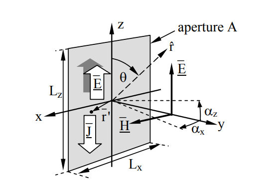
The electric field \( \mathrm{\hat{z} \underline{E}_{0} \equiv \overline{\underline E}_{0}}\) must satisfy the boundary condition (2.6.11) that:

\[\overline{\mathrm{\underline J}}_{\mathrm{S}}=\hat{y} \times\left[\overline{\mathrm{\underline H}}\left(\mathrm{y}=0_{+}\right)-\overline{\mathrm{\underline H}}\left(\mathrm{y}=0_{-}\right)\right]=\hat{y} \times\left[\hat{x} \frac{\mathrm{\underline E}_{0}}{\eta_{\mathrm{o}}}+\hat{x} \frac{\mathrm{\underline E}_{0}}{\eta_{\mathrm{o}}}\right]\]

\[\overline{\mathrm{\underline J}}_{\mathrm{S}}=-\hat{z} 2 \frac{\mathrm{\underline E}_{0}}{ \underline{\eta_{\mathrm{o}}}}=-2 \frac{\overline{\mathrm{\underline E}}_{0}}{\eta_{\mathrm{o}}}\left[\mathrm{Am}^{-1}\right]\]

Therefore we can consider any plane wave emerging from an aperture as emanating from an equivalent current sheet \( \underline{\mathrm{\overline J}}_{\mathrm{\underline S}}\) given by (11.1.4) provided we neglect radiation from the charges and currents induced at the aperture edges. They can generally be neglected if the aperture is large compared to a wavelength and if we remain close to the y axis in the direction of propagation, because then the aperture area dominates the observable radiating area. This approximation (11.1.4) for a finite aperture is valid even if the strength of the plane wave varies across the aperture slowly relative to a wavelength.

The equivalent current sheet (11.1.4) radiates according to (11.1.5) [from (10.2.8)], where we represent the current sheet by an equivalent array of Hertzian dipoles of length dz and current \( \mathrm{\overline{\underline I}=\underline{\overline J}_{s} d x}\):

\[\overline{\mathrm{\underline E}}=\hat{\theta} \frac{\mathrm{jk} \mathrm{\underline{I}d} \eta_{\mathrm{o}}}{4 \pi \mathrm{r}} \mathrm{e}^{-\mathrm{j} \mathrm{kr}} \sin \theta \qquad \qquad \qquad \text{(far-field radiation) }\]

The far fields radiated by the z-polarized current sheet \( \mathrm{\overline{\mathrm{\underline J}}_S (x,z)}\) in the aperture A are then:

\[\begin{align}\overline{\mathrm{\underline E}}_{\mathrm{ff}}(\theta, \phi) & \cong \hat{\theta} \frac{\mathrm{j} \eta_{\mathrm{o}}}{2 \lambda \mathrm{r}} \sin \theta \int_{\mathrm{A}} \underline{\mathrm{J}}_{\mathrm{Z}}(\mathrm{x}, \mathrm{z}) \mathrm{e}^{-\mathrm{j} \mathrm{kr}(\mathrm{x}, \mathrm{z})} \mathrm{d} \mathrm{x} \ \mathrm{dz} \nonumber \\& \cong-\hat{\theta} \frac{\mathrm{j}}{\lambda \mathrm{r}} \sin \theta \int_{\mathrm{A}} \mathrm{\underline E}_{\mathrm{o}}(\mathrm{x}, \mathrm{y}) \mathrm{e}^{-\mathrm{j} \mathrm{kr}(\mathrm{x}, \mathrm{z})} \mathrm{dx} \ \mathrm{dz}\end{align}\]

To simplify the integral we can assume all rays are parallel by using the Fraunhofer far-field approximation:

\[\mathrm{e}^{-\mathrm{j} \mathrm{kr}(\mathrm{x}, \mathrm{z})} \cong \mathrm{e}^{-\mathrm{j} \mathrm{kr}_{\mathrm{o}}} \mathrm{e}^{+\mathrm{j} \mathrm{k} \hat{r} \bullet \mathrm{r}^{\prime}} \qquad\qquad\qquad(\textit{Fraunhofer approximation})\]

where we define position within the aperture \( \overline{\mathrm{r}}^{\prime} \equiv \mathrm{x} \hat{x}+\mathrm{z} \hat{z}\), and the distance \( \mathrm{r_{0}=\left(x^{2}+y^{2}+z^{2}\right)^{0.5}}\). The Fraunhofer approximation is generally used when \( \mathrm{r}_{\mathrm{o}}>2 \mathrm{L}^{2} / \lambda\). Then:

\[\overline{\mathrm{\underline E}}_{\mathrm{ff}}(\theta, \phi) \cong-\hat{\theta} \frac{\mathrm{j}}{\lambda \mathrm{r}} \mathrm{e}^{-\mathrm{j} \mathrm{kr}_{\mathrm{o}}} \sin \theta \int_{\mathrm{A}} \mathrm{\underline E}_{\mathrm{oz}}(\mathrm{x}, \mathrm{z}) \mathrm{e}^{+j k \hat{r} \bullet \mathrm {\overline r}^\prime} \mathrm{dx} \ \mathrm{dz}\]

Those points in space too close to the aperture for the Fraunhofer approximation to apply lie in the Fresnel region where r < ~ 2L²/λ, as shown in (11.1.4). If we restrict ourselves to angles close to the y axis we can define the angles \( \alpha_{\mathrm x}\) and \( \alpha_{\mathrm z}\) from the y axis in the x and z directions, respectively, as illustrated in Figure 11.1.1, so that:

\[\mathrm{\hat{r} \bullet \bar{r}^{\prime} \cong x \sin \alpha_{x}+z \sin \alpha_{z} \cong x \alpha_{x}+z \alpha_{z}}\]

Therefore, close to the y axis (11.1.8) can be approximated⁵⁵ as:

\[\overline{\mathrm{\underline E}}_{\mathrm{ff}}\left(\alpha_{\mathrm{x}}, \alpha_{\mathrm{z}}\right) \cong-\hat{\theta} \frac{\mathrm{j}}{\lambda \mathrm{r}} \mathrm{e}^{-\mathrm{j} \mathrm{kr}_{\mathrm{o}}} \int_{\mathrm{A}} \mathrm{\underline E}_{\mathrm{oz}}(\mathrm{x}, \mathrm{z}) \mathrm{e}^{+\mathrm{j} 2 \pi\left(\mathrm{x} \alpha_{\mathrm{x}}+\mathrm{z} \alpha_{\mathrm{z}}\right) / \lambda} \mathrm{dx} \ \mathrm{dz}\]

which is the Fourier transform of the aperture field distribution \(\mathrm{\underline{E}_{o z}(x, z)} \), times a factor that depends on distance r and wavelength λ. Unlike the usual Fourier transform for converting signals between the time and frequency domains, this reversible transform in (11.1.10) is between the aperture spatial domain and the far-field angular domain.

⁵⁵ In the Huygen’s approximation a factor of (1 + cos\(\alpha\))/2 is added to improve the accuracy, but this has little impact near the y axis. In this expression α is the angle from the direction of propagation (y axis) in any direction.

For reference, the Fourier transform for signals is:

\[\mathrm{\underline{S}(f)=\int_{-\infty}^{\infty} s(t) e^{-j 2 \pi f t} d t}\]

\[\mathrm{s(t)=\int_{-\infty}^{\infty} \underline{S}(f) e^{j 2 \pi f t} d f}\]

The Fourier transform (11.1.11) has exactly the same form as the integral of (11.1.10) if we replace the aperture coordinates x and z with their wavelength-normalized equivalents x/λ and z/λ, analogous to time t; α is analogous to frequency f.

Assume the aperture of Figure 11.1.1 is z-polarized, has dimensions \(\mathrm{L}_{\mathrm{x}} \times \mathrm{L}_{\mathrm{z}}\), and is uniformly illuminated with amplitude \(\mathrm{\underline E}_{0}\). Then its far fields can be computed using (11.1.10):

\[\underline{\mathrm{\overline E}}_{\mathrm{ff}}\left(\alpha_{\mathrm{x}}, \alpha_{\mathrm{z}}\right) \cong-\hat{\theta} \frac{\mathrm{j}}{\lambda \mathrm{r}} \mathrm{e}^{-\mathrm{j} \mathrm{kr}_{\mathrm{o}}} \int_{-\mathrm{L}_{\mathrm{z}} / 2}^{+\mathrm{L}_{\mathrm{z}} / 2} \mathrm{e}^{+\mathrm{j} 2 \pi \alpha_{\mathrm{z}} \mathrm{z} / \lambda} \int_{-\mathrm{L}_{\mathrm{x}} / 2}^{+\mathrm{L}_{\mathrm{x}} / 2} \underline{\mathrm{E}}_{\mathrm{o}}(\mathrm{x}, \mathrm{z}) \mathrm{e}^{+\mathrm{j} 2 \pi \alpha_{\mathrm{x}} \mathrm{x} / \lambda} \mathrm{dx} \ \mathrm{dz}\]

The inner integral yields:

\[\begin{align}\int_{-\mathrm{L}_{\mathrm{x}} / 2}^{+\mathrm{L}_{\mathrm{x}} / 2} \mathrm{\underline E}_{\mathrm{o}}(\mathrm{x}, \mathrm{z}) \mathrm{e}^{+\mathrm{j} 2 \pi \alpha_{\mathrm{x}} \mathrm{x} / \lambda} \mathrm{dx} &=\mathrm{\underline E}_{\mathrm o} \frac{\lambda}{\mathrm{j} 2 \pi \alpha_{\mathrm{x}}}\left[\mathrm{e}^{+\mathrm{j} \pi \alpha_{\mathrm{x}} \mathrm{L}_{\mathrm{x}} / \lambda}-\mathrm{e}^{-\mathrm{j} \pi \alpha_{\mathrm{x}} \mathrm{L}_{\mathrm{x}} / \lambda}\right] \nonumber \\&=\mathrm{\underline E}_{\mathrm{o}} \frac{\sin \left(\pi \alpha_{\mathrm{x}} \mathrm{L}_{\mathrm{x}} / \lambda\right)}{\pi \alpha_{\mathrm{x}} / \lambda}\end{align}\]

The outer integral yields a similar result, so the far field is:

\[\overline{\mathrm{\underline E}}_{\mathrm{ff}}(\theta, \phi) \cong-\hat{\theta} \frac{\mathrm{j}}{\lambda \mathrm{r}} \mathrm{\underline E}_{\mathrm{oz}} \mathrm{e}^{-\mathrm{j} \mathrm{kr}_{\mathrm{o}}} \bullet \mathrm{L}_{\mathrm{x}} \mathrm{L}_{\mathrm{z}} \frac{\sin \left(\pi \alpha_{\mathrm{x}} \mathrm{L}_{\mathrm{x}} / \lambda\right)}{\pi \alpha_{\mathrm{x}} \mathrm{L}_{\mathrm{x}} / \lambda} \frac{\sin \left(\pi \alpha_{\mathrm{z}} \mathrm{L}_{\mathrm{z}} / \lambda\right)}{\pi \alpha_{\mathrm{Z}} \mathrm{L}_{\mathrm{z}} / \lambda}\]

The total power P_t radiated through the aperture is simply \(\mathrm{A}\left|\mathrm{\underline E}_{\mathrm{o}}\right|^{2} / 2 \eta_{\mathrm{o}} \), where A = L_xL_z, so the antenna gain \(\mathrm{G}\left(\alpha_{\mathrm{X}}, \alpha_{\mathrm{Z}}\right)\) given by (10.3.1) is:

\[\begin{align}
\mathrm{G}\left(\alpha_{\mathrm{x}}, \alpha_{\mathrm{z}}\right) & \cong \frac{\left|\mathrm{E}_{\mathrm{ff}}\left(\alpha_{\mathrm{x}}, \alpha_{\mathrm{z}}\right)\right|^{2} / 2 \eta_{\mathrm{o}}}{\mathrm{P}_{\mathrm{t}} / 4 \pi \mathrm{r}^{2}} \\
& \cong \mathrm{A} \frac{4 \pi}{\lambda^{2}}\left(\frac{\sin ^{2}\left(\pi \alpha_{\mathrm{x}} \mathrm{L}_{\mathrm{x}} / \lambda\right)}{\left(\pi \alpha_{\mathrm{x}} \mathrm{L}_{\mathrm{x}} / \lambda\right)^{2}}\right)\left(\frac{\sin ^{2}\left(\pi \alpha_{\mathrm{z}} \mathrm{L}_{\mathrm{z}} / \lambda\right)}{\left(\pi \alpha_{\mathrm{z}} \mathrm{L}_{\mathrm{z}} / \lambda\right)^{2}}\right)
\end{align}\]

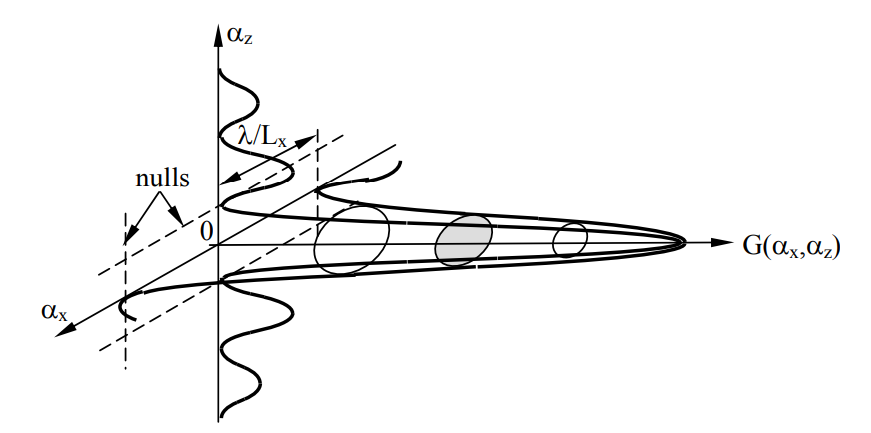
The function (sin x)/x appears so often in electrical engineering that it has its own symbol ‘sinc(x)’. Note that sinc(0) = 1 since \(\mathrm{\sin (x) \cong x-\left(x^{3} / 6\right) \text { for } x<<1} \). This gain pattern is plotted in Figure 11.1.2. The first nulls occur when \(\pi \alpha_{1} \mathrm{L}_{\mathrm{i}} / \lambda=\pi \) (i = x or z), and therefore \(\alpha_{\text {null }}=\lambda / \mathrm{L} \) where a narrower beamwidth α corresponds to a wider aperture L. The on-axis gain is:

\[\mathrm{G}(0,0)=\frac{4 \pi}{\lambda^{2}} \mathrm{A} \qquad \qquad \qquad \text{(gain of uniformly illuminated aperture area A) }\]

Equation (11.1.18) applies to any uniformly illuminated aperture antenna, and such antennas have on-axis effective areas A(θ,\(\phi\)) that approach their physical areas A, and have peak gains \(\mathrm{G}_{\mathrm{o}}=4 \pi \mathrm{A} / \lambda^{2} \). The antenna pattern of Figure 11.1.2 vaguely resembles that of circular apertures as well, and the same nominal angle to first null, λ/L, roughly applies to all. Such diffraction pattterns largely explain the limiting angular resolution of telescopes, cameras, animal eyes, and photolithographic equipment used for fabricating integrated circuits.

Figure \(\PageIndex{2}\): Antenna gain for uniformly illuminated rectangular aperture.

The coupling between two facing aperture antennas having effective areas A₁ and A₂ is:

\[\mathrm{P_{r_{2}}=\frac{P_{t_{1}}}{4 \pi r^{2}} G_{1} A_{2}=\frac{P_{t_{1}}}{\lambda^{2} r^{2}} A_{1} A_{2}=P_{t_{1}}\left(\frac{\lambda}{4 \pi r}\right)^{2} G_{1} G_{2}}\]

where \( \mathrm{P_{r_{2}}}\) and \( \mathrm{P_{t_{1}}}\) are the power received by antenna 2 and the total power transmitted by antenna 1, respectively. For (11.1.19) to be valid, \(r^{2} \lambda^{2}>>A_{1} A_{2} \); if A₁ = A₂ = D² , then we require \(\mathrm{r}>>\mathrm{D}^{2} / \lambda\) for validity. Otherwise (11.1.19) could predict that more power would be received than was transmitted.

Example \(\PageIndex{A}\)

What is the angle between the first nulls of the diffraction pattern for a visible laser (λ = 0.5 microns) illuminating a 1-mm square aperture (about the size of a human iris)? What is the approximate diffraction-limited angular resolution of the human visual system? How does this compare to the maximum angular diameters of Venus, Jupiter, and the moon (~1, ~1, and ~30 arc minutes in diameter, respectively)?

Solution

The first null occurs at

\( \phi=\sin ^{-1}(\lambda / \mathrm{L}) \cong 5 \times 10^{-7} / 10^{-3}=5 \times 10^{-4} \ \text {radians }=0.029^{\circ} \cong 1.7 \ \text{arc}\) minutes.

This is 70 percent larger than the planets Venus and Jupiter at their points of closest approach to Earth, and ~6 percent of the lunar diameter. Cleverly designed neuronal connections in the human visual system improve on this for linear features, as can a dark-adapted iris, which has a larger diameter.

Example \(\PageIndex{B}\)

A cell-phone dipole antenna radiates one watt toward a uniformly illuminated square aperture antenna of area A = one square meter. If P_r = 10^-9 watts are required by the receiver for satisfactory link performance, how far apart r can these two terminals be? Does this depend on the shape of the aperture antenna if A remains constant?

Solution

\[ \mathrm{P_{r}=A P_{t} G_{t} / 4 \pi r^{2} \Rightarrow r=\left(A P_{t} G_{t} / 4 \pi P_{r}\right)^{0.5}=\left(1 \times 1 \times 1.5 / 4 \pi 10^{-9}\right)^{0.5} \cong 10.9 \ \mathrm{km}}\]

The on axis gain G_t of a uniformly illuminated constant-phase aperture antenna is given by (11.1.18). The denominator depends only on the power transmitted through the aperture A, not on its shape. The numerator depends only on the on-axis far field E_ff, given by (11.1.10), which again is independent of shape because the phase term in the integral is unity over the entire aperture. Since the on-axis gain is independent of aperture shape, so is the effective area A since \(\mathrm{A}(\theta, \phi)=\mathrm{G}(\theta, \phi) \lambda^{2} / 4 \pi \). The on-axis effective area of a uniformly illuminated aperture approximates its physical area.

Common aperture antennas

Section 11.1.2 derived the basic equation (11.1.10) that characterizes the far fields radiated by aperture antennas excited with z-polarized electric fields \( \mathrm{\overline{\underline E}_{0}(x, z)=\hat{z} \underline{E}_{0 z}(x, z)}\) in the x-z aperture plane:

\[\overline{\mathrm{\underline E}}_{\mathrm{ff}}(\theta, \phi) \cong \hat{\theta} \frac{\mathrm{j}}{\lambda \mathrm{r}} \sin \theta \mathrm{e}^{-\mathrm{jkr}} \oiint_{\mathrm{A}} \mathrm{E}_{\mathrm{oz}}(\mathrm{x}, \mathrm{z}) \mathrm{e}^{\mathrm{jk} \hat{\mathrm{r}} \bullet \overline{\mathrm{r}^{\prime}}} \mathrm{dx} \ \mathrm{dz}\]

The unit vector \( \hat{\mathrm{r}}\) points from the antenna toward the receiver and \(\overline{\mathrm r^{\prime}} \) is a vector that locates \(\overline{\mathrm{\underline E}}_{\mathrm o}\left(\mathrm{r}^{\prime}\right) \) within the aperture. This expression assumes the receiver is sufficiently far from the aperture that a single unit vector \(\hat{\mathrm{r}} \) suffices for the entire aperture and that the receiver is therefore in the Fraunhofer region. The alternative is the near-field Fresnel region where \(r< 2D^2/λ\), as discussed in Section 11.1.4; D is the aperture diameter. It also assumes the observer is close to the axis perpendicular to the aperture, say within ~40°. The Huygen’s approximation extends this angle further by replacing sinθ with (1 + cosβ)/2, where θ is measured from the polarization axis and β is measured from the y axis:

\[\overline{\mathrm{\underline E}}_{\mathrm{ff}}(\theta, \phi) \cong \hat{\theta} \frac{\mathrm{j}}{2 \lambda \mathrm{r}}(1+\cos \beta) \mathrm{e}^{-\mathrm{j} \mathrm{kr}} \oiint_{\mathrm{A}} \mathrm{\underline E}_{\mathrm{oz}}(\mathrm{x}, \mathrm{z}) \mathrm{e}^{-\mathrm{j} \mathrm{k} \hat{\mathrm{r}} \bullet \mathrm{\overline r}^{\prime}} \text { dx dz } \qquad \qquad \qquad (\textit {Huygen's approximation})\]

Evaluating the on-axis gain of a uniformly excited aperture of physical area A having \( \mathrm{\underline{E}_{o z}(x, z)=E_{o z}}\) is straightforward when using (11.1.21) because the exponential factor in the integral is unity within the entire aperture. The gain follows from (11.1.16). The results are:

\[\overline{\mathrm{\underline E}}_{\mathrm{ff}}(0,0) \cong \hat{\theta} \frac{\mathrm{j}}{\lambda \mathrm{r}} \mathrm{e}^{-\mathrm{j} \mathrm{kr}} \oiint_{\mathrm{A}} \mathrm{\underline E}_{\mathrm{oz}} \mathrm{dx} \ \mathrm{dz} \qquad \qquad \qquad \text { (on-axis field) }\]

\[\mathrm{G}(0,0)=\frac{|\overline{\mathrm{\underline E}}_\mathrm{ff}(0,0)|^{2} / 2 \eta_{\mathrm{o}}}{\mathrm{P}_{\mathrm{T}} / 4 \pi \mathrm{r}^{2}} \qquad \qquad \qquad \text{(on-axis gain) }\]

But the total power P_T transmitted through the aperture area A can be evaluated more easily than the alternative of integrating the radiated intensity I(θ,φ) over all angles. The intensity I within the aperture is \( \left|\overline{\mathrm{\underline E}}_{\mathrm{oz}}\right|^{2} / 2 \eta_{\mathrm{o}}\), therefore:

\[\mathrm{P}_{\mathrm{T}}=\frac{\left|\overline{\mathrm{\underline E}}_{\mathrm{oz} }\right|^{2}}{2 \eta_{\mathrm{o}}} \mathrm{A}\]

Then substitution of (11.1.22) and (11.1.24) into (11.1.23) yields the gain of a uniformly illuminated lossless aperture of physical area A:

\[\mathrm{G}(0,0)=\frac{(\lambda \mathrm{r})^{-2}\left(\mathrm{E}_{\mathrm{oz}} \mathrm{A}\right)^{2} / 2 \eta_{\mathrm{o}}}{\left(\mathrm{E}_{\mathrm{oz}}^{2} / 2 \eta_{\mathrm{o}}\right) \mathrm{A} / 4 \pi \mathrm{r}^{2}}=\frac{\lambda^{2}}{4 \pi} \mathrm{A} \qquad \qquad \qquad \text { (gain of uniform aperture) }\]

The off-axis gain of a uniformly illuminated aperture depends on its shape, although the on-axis gain does not.

Perhaps the most familiar radio aperture antennas are parabolic dishes having a point feed that radiates energy toward a parabolic mirror so as to produce a planar wave front for transmission, as suggested in Figure 11.1.3(a). Conversely, incoming radiation is focused by the mirror on the antenna feed, which intercepts and couples it to a transmission line connected to the receiver. Typical focal lengths (labeled “f” in the figure) are ~half the diameter D for radio systems, and are often much longer for optical mirrors that produce images.

Figure \(\PageIndex{3}\): Aperture antennas and angle of first null.

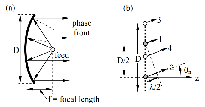
Figure 11.1.3(b) suggests the angle \( \theta_{\mathrm{n}}\) at which the first null of a uniformly illuminated rectangular aperture of width D occurs; it is the angle at which all the phasors emanating from each point on the aperture integrate in (11.1.10) to zero. In this case it is easy to pair the phasors originating D/2 apart so each pair cancels at \( \theta_{\mathrm{n}}\). For example, radiation from aperture element 2 has to travel λ/2 farther than radiation from element 1 and therefore they cancel each other. Similarly radiation from elements 3 and 4 cancel, and the sum of all such pairs cancel at the null angle:

\[\theta_{\mathrm{n}}=\sin ^{-1}(\lambda / \mathrm{D}) \ [\text { radians }]\]

where \(\theta_{\mathrm n} \cong \lambda / D \) for λ/D << 1.

Approximately the same null angle results for uniformly illuminated circular apertures, for which integration yields \(\theta_{\mathrm{n}} \cong 1.2 \lambda / \mathrm{D} \). Consider the human eye, which has a pupil that normally is ~2 mm in diameter, but can dilate to ~1 cm in the dark. For a wavelength of 5×10^-7 meters, we find the normal diffraction-limited angular resolution of the eye is ~λ/D = 5×10^-7/(2×10^-3) = 2.5×10^-4 radians or ~0.014 degrees, or ~0.9 arc minutes. For comparison, the planets Venus and Jupiter are approximately 1 arc minute in diameter at closest approach, and the moon and sun are approximately 30 arc minutes in diameter.

A large astronomical telescope like the 200-inch system at Palomar has a nominal diffraction limit of \( \lambda / \mathrm{D} \cong 5 \times 10^{-7} / 5.08 \cong 10^{-7}\) radians or ~0.02 arc seconds, where there are 60 arc seconds in an arc minute, and 60 arc minutes in a degree. This is adequate to resolve an automobile on the moon. Unfortunately mirror surface imperfections, focus misplacement, and atmospheric turbulence limit the actual angular resolution of Palomar to ~1 arc second on the very best nights; normal daytime turbulence is far worse.

Practical issues generally shape the design of parabolic radio antennas. First, mechanical (gravity and wind) and thermal issues (temperature gradients) usually limit their angular resolution to ~1 arc minute; most antennas are too small relative to λ to achieve this resolution, however. Second, the antenna feed that illuminates the parabola tends to spray its radiation in a broad pattern that extends past the edge of the reflector creating backlobes. Third, the finite extent of the aperture results in an antenna pattern with sidelobes and unwanted responsiveness to directions beyond the main lobe.

Equation (11.1.10) showed how the angular dependence of the far-fields of an aperture was proportional to the Fourier transform of the aperture excitation function. For example, (11.1.17) and Figure 11.1.2 showed the radiation pattern of a uniformly illuminated aperture measuring L_x by L_z. Significant energy was radiated beyond the first nulls at \(\mathrm{\alpha_{x}=\lambda / L_{x}}\) and \( \mathrm{\alpha_{z}=\lambda / L_{z}}\). A finite aperture necessarily radiates something at all angles, just as a finite voltage pulse in a circuit has at least some energy at all frequencies; the sharper the pulse edges, the more high-frequency content they have. Therefore, reducing the sharp discontinuities in field strength at the aperture edge, a strategy called tapering, can reduce diffraction sidelobes. Antenna feeds are typically designed to reduce field strengths by factors of 2-4 at the mirror edges for this reason, but the resulting effective reduction in aperture diameter produces a slightly broader main lobe, just as the Fourier transform of a narrower pulse produces a broader spectral band.

A final consideration is sometimes important when designing aperture antennas, and that involves aperture blockage, which results when transmitted radiation reflected from the mirror is blocked or scattered by the antenna feed at the focus of the parabola. Not only does the scattered radiation contribute to side or back lobes, but it also is lost to the main beam. Example 11.1C illustrates these issues.

Example \(\PageIndex{C}\)

A uniformly illuminated square aperture is 1000 wavelengths long on each side. What is its antenna gain \( \mathrm{G}\left(\alpha_{\mathrm{x}}, \alpha_{\mathrm{z}}\right)\) for α << 1? What is the gain G_o' if the center of this fully illuminated aperture is blocked by a square absorber 100 wavelengths on a side? What is the extent and approximate magnitude of the sidelobes introduced by the blockage?

Solution

The on-axis gain \(\mathrm{G}_{\mathrm{o}}=\mathrm{A} 4 \pi / \lambda^{2}=1000^{2} \times 4 \pi \). The angular dependence is proportional to the square of the far-field, \( \left|\mathrm{E}\left(\alpha_{\mathrm{x}}, \alpha_{\mathrm{z}}\right)\right|^{2}\), where the far field is the Fourier transform of the aperture field distribution. The full solution for \( \mathrm{G}\left(\alpha_{\mathrm{x}}, \alpha_{\mathrm{z}}\right)\) is developed in Equations (11.1.13–17). If the blocked portion of the aperture is illuminated so the energy there is absorbed, then the total transmitted power P_t in the expression (11.1.16) for gain is unchanged, while the area over which \( \overline{\mathrm{\underline E}}_{\mathrm{ff}}^{\prime}\) is integrated in (11.1.13) is reduced by the 1 percent blockage (100² is 1 percent of 1000²). Therefore \( \left|\overline{\mathrm{\underline E}}_{\mathrm{ff}}^{\prime}(0,0)\right|^{2}\), the numerator of (11.1.16), and G_o'(0,0) are all reduced by a factor of 0.99² ≅ 0.98. Thus G_o' ≅ 0.98 G_o. If the blocked portion of the aperture were not illuminated so as to avoid the one percent absorption, then G_o'(0,0) would be reduced by only 1 percent: \( \mathrm{G}_{\mathrm{o}}^{\prime}=\mathrm{A}^{\prime} 4 \pi / \lambda^{2}\). The sidelobes for the blocked aperture follow from the Fourier transform (11.1.13), where the aperture excitation E_o(x,z) is the sum of a positive square “boxcar” function 1000λ on a side, and a negative square boxcar 100λ on a side. Since this transform is linear, \( \overline{\mathrm{E}}_{\mathrm{ff}}\left(\alpha_{\mathrm{x}}, \alpha_{\mathrm{z}}\right)\) is the sum of the transforms of the positive and negative boxcar functions, and the antenna sidelobes therefore have contributions from each. Most important is the main lobe of the diffraction pattern of the smaller “blockage” boxcar, which has magnitude ~0.01² that of G_o', and a halfpower beamwidth \(\theta_{\mathrm{BB}} \) that is 10 times greater than the main lobe of the larger boxcar: \( \theta_{\mathrm{BB}} \cong \lambda / \mathrm{D}_{\mathrm{B}}=\lambda / 100 \lambda\). The total antenna pattern is the square of the summed transforms and more complicated; the innermost few sidelobes are approximately those of the original antenna, while the blockage-induced sidelobes are more important at greater angles.

Near-field diffraction and Fresnel zones

Often receivers are sufficiently close to the source that the Fraunhofer parallel-ray approximation of (11.1.7) is invalid. Then the Huygen’s approximation (11.1.21) can be used:

\[\overline{\mathrm{\underline E}}_{\mathrm{ff}} \cong \hat{\theta} \frac{\mathrm{j}}{2 \lambda_{\mathrm{r}}}(1+\cos \beta) \oiint_{\mathrm{A}} \mathrm{\underline E}_{\mathrm{oz}}(\mathrm{x}, \mathrm{z}) \mathrm{e}^{-\mathrm{j} \mathrm{k} \mathrm{r}(\mathrm{x}, \mathrm{y})} \mathrm{dx} \ \mathrm{dz} \qquad\qquad\qquad \text { (Huygen's approximation) }\]

for which the distance between the receiver and the point x,y in the aperture is defined as r(x,y). This region close to a source or obstacle where the Fraunhofer approximation is invalid is called the Fresnel region.

If the phase of \( \underline{\mathrm{E}}_{\mathrm{oz}}\) in the source aperture is constant everywhere, then contributions to \( \mathrm{\underline E}_{\mathrm{ff}}(0,0)\) from some parts of the aperture will tend to cancel contributions from other parts because they are out of phase. For example, contributions from the central circular zone where r(x,y) ranges from r_o to r_o + λ/2 will largely cancel the contributions from the surrounding ring where r(x,y) ranges from r_o + λ/2 to r_o + λ; it is easily shown that these two rings have approximately the same area, as do all such rings over which the delay varies by λ/2.⁵⁶ Such rings are illustrated in Figure 11.1.4(a)

⁵⁶ The area of the inner circle (radius a) is \(\mathrm{\pi a^{2}=\pi\left[\left(r_{0}+\lambda / 2\right)^{2}-r_{0}^{2}\right] \cong \pi r_{0} \lambda}\) if λ << 2r_o. The area of the immediately surrounding Fresnel ring (radius b) is \(\mathrm{\pi\left(b^{2}-a^{2}\right)=\pi\left[\left(r_{0}+\lambda\right)^{2}-r_{0}^{2}\right]-\pi\left[\left(r_{0}+\lambda / 2\right)^{2}-r_{0}^{2}\right] \cong \pi r_{0} \lambda}\), subject to the same approximation. Similarly, all other Fresnel rings can be shown to have approximately the same area if λ << 2r_o.

Figure \(\PageIndex{4}\): Fresnel zone plate.

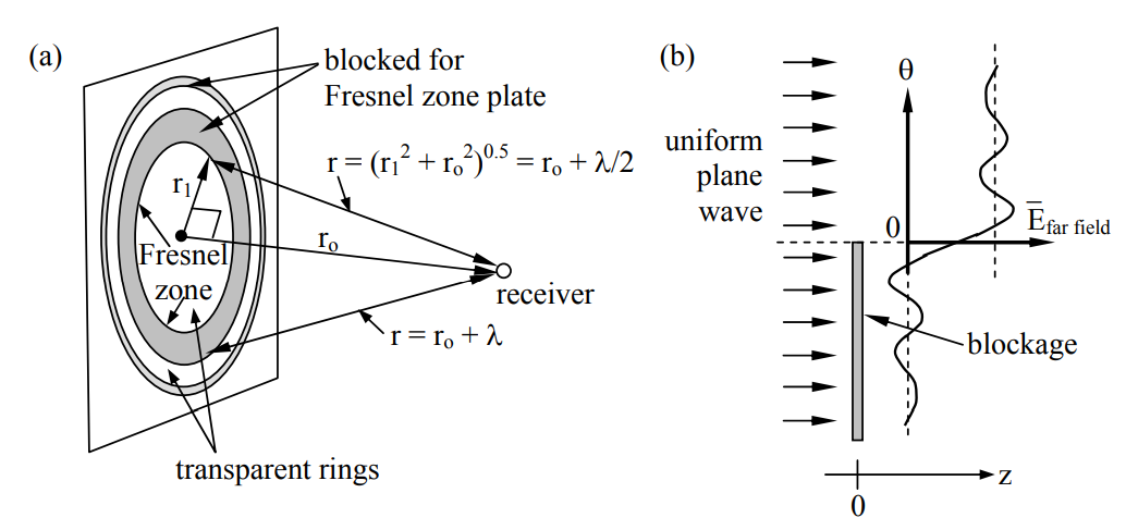
One technique for maximizing diffraction toward an observer is therefore simply to physically block radiation from those alternate zones contributing negative fields, as suggested in Figure 11.1.4(a). Such a blocking device is called a Fresnel zone plate. The central ring having positive phase is called the Fresnel zone. Note that if only the central zone is permitted to pass, the received intensity is maximum, and if the first two zones pass, the received intensity is nearly zero because they have approximately the same area. The second zone is weaker, however, because r and θ are larger. Three zones can yield nearly the same intensity as the first zone alone because two of the three zones nearly cancel, and so on. By blocking alternate zones the received intensity can be many times greater than if there were no blockage at all. Thus a multiring zone plate acts as a lense by focusing energy received over a much larger area than would be intercepted by the receiver alone. This type of lense is particularly valuable for focusing very short-wave radiation such as x-rays which are difficult to reflect or diffract using traditional mirrors or lenses.

Another advantage of zone plate lenses is that they can be manufactured lithographically, and their critical dimensions are usually many times larger than the wavelengths involved. For example, an x-ray zone plate designed to operate at λ = 10^-8 [m] at a distance r_o of one centimeter will have a central zone of diameter \(2\left[\left(\mathrm{r}_{0}+\lambda / 2\right)^{2}-\mathrm{r}_{0}^{2}\right]^{0.5} \cong 2\left(\mathrm{r}_{0} \lambda\right)^{0.5}=2 \times 10^{-5} \) meters, a dimension easily fabricated using modern semiconductor lithographic techniques.

Another example of diffraction is wireless communications in urban environments, which often involves line-of-sight reception of waves past linear obstacles slightly to one side or slightly obscuring the source. Again Huygen’s equation (11.1.27) can be used to determine the result. Referring to Figure 11.1.4(b), if there is no blockage, traditional equations can be used to compute the received intensity. If exactly half the path is blocked by a wall obscuring the bottom half of the illuminated aperture, for example, then the integral in (11.1.27) will yield exactly half the previous value of E_ff, and the power (proportional to E_ff²) will be reduced by a factor of four, or ~6dB. If the observer moves up or down less than ~half the radius of the Fresnel zone, then the received power will vary only modestly. For example, an FM radio (say 10⁸ Hz) about 100 meters beyond a tall wide metal wall can have a line of sight that passes through the wall a distance of ~(rλ)^0.5/2 = 17 meters below its top without suffering great loss; (rλ)^0.5 is the radius of the Fresnel zone. Conversely, a line-of-sight that passes less than ~17 meters above the top of the wall will also experience modest diffractive effects.

The Fresnel region approximately begins when the central ray arrives at distance r_o, more than λ/16 ahead of rays from the perimeter of an aperture of diameter D. That is:

\[\mathrm{\sqrt{\left(\frac{D}{2}\right)^{2}+r_{0}^{2}}-r_{0} \ \tilde{>} \ \frac{\lambda}{16}}\]

For D << R this becomes:

\[\mathrm{r}_{\mathrm{o}}\left(\sqrt{\left(\frac{\mathrm{D}}{2 \mathrm{r}_{\mathrm{o}}}\right)^{2}+1}-1\right) \cong \frac{\mathrm{D}^{2}}{8 \mathrm{R}} \ \tilde{>} \ \frac{\lambda}{16}\]

Therefore the Fresnel region is:

\[\mathrm{r}_{\mathrm{o}} \ \tilde{<} \ \frac{2 \mathrm{D}^{2}}{\lambda} \qquad \qquad \qquad \text{(Fresnel region)}\]