11.2: Wire Antennas

Introduction to Wire Antennas

Exact solution of Maxwell’s equations for antennas is difficult because antennas typically have complex shapes for which it is difficult to match boundary conditions. Often complex wave expansions with many degrees of freedom are required, and even modern software tools can be challenged. Fortunately, most common wire antennas permit their current distributions to be guessed accurately relative to the given terminal current, as explained in Section 11.2.2. Once the current distribution is known everywhere, the radiated fields, radiation and dissipative resistance, antenna gain, and antenna effective area can be calculated. If the antenna is used at a frequency far from resonance, the reactance can also be estimated.

If the antenna is small compared to a wavelength λ then its current distribution \(\underline{\mathrm I} \) and the open-circuit voltage \( \underline{\mathrm{V}}_{\mathrm{Th}}\) can be determined using the quasistatic approximation. If the current distribution is known, then the radiated far-fields \(\overline{\mathrm{\underline E}}_{\mathrm{ff}} \) can be computed using (10.2.8) by integrating the contributions \( \Delta \underline{\mathrm{\overline E}}_{\mathrm{ff}}\) from each short current element \(\mathrm{\underline{I}d} \) (d is the element length and is replaced by ds in the integral), where:

\[\Delta \overline{\mathrm{\underline E}}_{\mathrm{ff}}=\hat{\theta} \frac{\mathrm{j} \mathrm{k} \mathrm{\underline{I}d} \eta_{\mathrm{o}}}{4 \pi \mathrm{r}} \mathrm{e}^{-\mathrm{j} \mathrm{kr}} \sin \theta \label{11.2.1}\]

\[\overline{\mathrm{\underline E}}_{\mathrm{ff}} \cong \frac{\mathrm{jk} \eta_{\mathrm{o}}}{4 \pi \mathrm{r}} \int_{\mathrm{S}}{\hat{\theta}} \underline{\mathrm{I}}(\mathrm{s}) \mathrm{e}^{-\mathrm{j} \mathrm{kr}} \sin \theta \mathrm{d} \mathrm{s} \label{11.2.2}\]

For antennas small compared to λ the factor before the integral of (\ref{11.2.2}) is nearly constant over the integrated length S, so average values suffice. If the wires run in more than one direction, the definition of \(\hat{\theta} \) and θ must change accordingly; θ is defined by the local angle between \( \overline{\underline{\mathrm I}}\) and \( \hat{\mathrm{r}}\), where \(\hat{\mathrm{r}} \) is the unit vector pointing from the antenna to the observer, as suggested in Figure 10.2.3. Equation \ref{11.2.2}, not surprisingly, reduces to Equation \ref{11.2.1} for a short straight wire carrying constant current \(\underline{\mathrm I} \) over a distance \(\mathrm d \ll λ\).

Once the radiated fields are known for a given antenna input current \(\underline{\mathrm I} \), the radiated intensity can be integrated over a sphere surrounding the antenna to yield the total power radiated P_R and the radiation resistance R_r, which usually dominates the resistive component of the antenna impedance and corresponds to power lost through radiation (10.3.16). The radiation resistance is simply related to P_R:

\[\mathrm{R}_{\mathrm{r}}=\frac{2 \mathrm{P}_{\mathrm{R}}}{| \mathrm{\underline I}^{2}|} \ [\text { ohms }] \qquad \qquad \qquad \text{(radiation resistance) } \label{11.2.3}\]

The open-circuit voltage can also be easily estimated for wire antennas small compared to λ. For example, the open-circuit voltage induced across a short dipole antenna shown in Figure 10.3.1 is simply the projection of the incident electric field \( \overline{\mathrm{E}}\) on the electrical centers of the two metallic structures comprising the dipole, and Example 10.3D showed how the open-circuit voltage across a loop antenna was proportional to the time derivative of the magnetic flux through it. In both cases the open-circuit voltage reveals the directional properties of the antenna. Computation of the radiation resistance requires knowledge of the radiated fields and integration of the radiated power over all angles, however. Equation (10.3.16) showed that the radiation resistance of a short dipole antenna of length d is \( \left(2 \pi \eta_{\mathrm{o}} / 3\right)(\mathrm{d} / \lambda)^{2}\) ohms. Slightly more complicated integrals over angles yield the radiation resistance for half-wave dipoles of length d and N-turn loop antennas of diameter d << λ: ~73 ohms and \( \sim 1.9 \times 10^{4} \mathrm{N}^{2}(\mathrm{d} / \lambda)^{4}\) ohms, respectively. The higher radiation resistance of loop antennas often makes them the antenna of choice when space is limited relative to wavelength, particularly when they are wound on a ferrite core (\( \mu \gg \mu_{0}\)) that increases their magnetic dipole moment.

Most wire antennas are not small compared to a wavelength, however, and the methods of the next section are then often used.

Current Distribution on Wires

The current distribution on wires is governed by Maxwell’s equations, which are most easily solved for simple geometries such as that of a coaxial cable, as discussed in Example 7.1B. The fields for a TEM wave in a coaxial cable are cylindrically symmetric and a function of radius r:

\[\overline{\mathrm{\underline E}}(\mathrm{r}, \mathrm{z})=\hat{\mathrm{r}} \underline{\mathrm{E}}_{0}(\mathrm{z}) / \mathrm{r} \ \left[\mathrm{V} \mathrm{m}^{-1}\right] \qquad \qquad \qquad \text{(coaxial cable electric field)} \label{11.2.4}\]

\[\overline{\mathrm{\underline H}}(\mathrm{r}, \mathrm{z})=\hat{\theta} \underline{\mathrm{H}}_{0}(\mathrm{z}) / \mathrm{r} \ \left[\mathrm{A} \mathrm{m}^{-1}\right] \qquad \qquad \qquad \text{(coaxial cable magnetic field)}^{57} \label{11.2.5}\]

⁵⁷ The magnetic field around a central wire, H = I/2\(\pi\)r, was given in (1.4.3).

The energy density and Poynting’s vector are proportional to field strength squared, so they decay as r^-2. Therefore the electromagnetic behavior of the line is dominated by the geometry near the central conductor where most of the electromagnetic energy is located, and the outer conductor can be deformed substantially before the fields near the center are significantly perturbed. For example, two-thirds of the power propagates within 10 cm of a 1-mm wire centered within a 1-meter outer cylinder, even though this represents only one-percent of the volume. This is easily shown by integrating the energy density from radius a to radius b, \( \mathrm{\int_{a}^{b} E_{o}^{2} r^{-2} 2 \pi r d r=2 \pi E_{o}^{2} \ln (b / a)}\), and comparing the results for different sub-volumes.

Therefore the fields near the axis of the coaxial cable illustrated in Figure 11.2.1(a) are altered but little if the outer conductor is replaced by a ground plane as illustrated in Figure 11.2.1(b), or even by a second wire, as shown in Figure 11.2.1(c). The significance of Figure 11.2.1 is therefore that current distributions on thin wire antennas closely resemble those on equivalent TEM lines, provided the lines are not so many wavelengths long that the energy is lost before it reaches the end, or so tightly bent that the segments induce strong voltages on their neighbors. This TEM approximation is valid for understanding the examples of this section.

A widely used antenna is the half-wave dipole, illustrated in Figure 11.2.1(d), which exhibits essentially no reactive impedance because the electric and magnetic energy storages approximately balance. The radiation resistance for any half-wave dipole in free space is ~73 ohms. Section 7.4.2 discusses how these energies balance in any TEM structure of length D = nλ/2 where n is an integer. Typical bandwidths Δω of a half-wave dipole are \(\Delta \omega / \omega_{\mathrm{o}}=1 / \mathrm{Q} \cong 0.1 \), where \( \mathrm{Q}=\omega_{\mathrm{o}} \mathrm{W}_{\mathrm{T}} / \mathrm{P}_{\mathrm{d}}\), as discussed in Section 7.4.3 and (7.4.4).

Figure \(\PageIndex{1}\): Fields near wire antennas resemble fields in TEM coaxial cables.

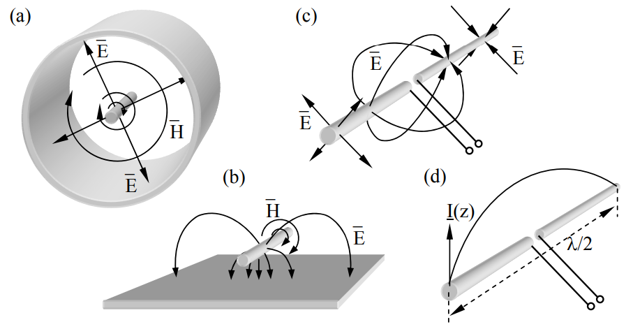
Figure 11.2.2 illustrates nominal current distributions on several antenna structures; these currents are consistent with those on comparable TEM lines propagating signals at the speed of light. The current distributions in the figure represent instantaneous distributions at the moment of current maximum.

Figure \(\PageIndex{2}\): Current distributions on wire antenna structures.

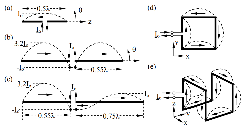
In these idealized cases the currents everywhere on the antenna approach zero one-quarter cycle later as the energy all converts from magnetic to electric. The voltage distributions when the currents are zero resemble those on the equivalent TEM lines, and are offset spatially by λ/4; at resonance the voltage peaks coincide with the current nulls. For example, the voltages and currents for Figure 11.2.2(a) resemble those of the open-circuited TEM resonator of Figure 7.4.1(a). The actual current and voltage distributions are slightly different from those pictured because radiation tends to weaken the currents farther from the antenna terminals, and because such free-standing or bent wires are not true TEM lines.

Figure 11.2.2(b) illustrates how terminal currents (I_o) can be made less than one-third the peak currents (3.2 I_o) flowing on the antenna simply by lengthening the two arms so they are each slightly longer than λ/2 so the current is close to a null at the terminals. Because smaller terminal currents thus correspond to larger antenna currents and radiated power, the effective radiation resistance of this antenna is increased well above the nominal 73 ohms of the half-wave dipole of (a). The reactance is slightly capacitive, however, and should be canceled with an inductor. Figure 11.2.2(c) illustrates how the peak currents can be made different in the two arms; note that the currents fed to the two arms must be equal and opposite, and this fact forces the two peak currents in the arms to differ. Figures (d) and (e) show more elaborate configurations, demonstrating that wire antennas do not have to lie in a straight line. The patterns for these antennas are discussed in the next section.

Antenna Patterns

Once the current distributions on wire antennas are known, the antenna patterns can be computed using (\ref{11.2.2}). Consider first the dipole antenna of Figure 11.2.2(a) and let its length be d, its terminal current be I_o′, and its maximum current be I_o. Then (\ref{11.2.2}) becomes:

\[\overline{\mathrm{\underline E}}_\mathrm{ff} \cong \frac{\mathrm{jk} \eta_{\mathrm{o}}}{4 \pi \mathrm{r}} \int_{-\mathrm{d} / 2}^{\mathrm{d} / 2} \hat{\theta} \underline{\mathrm{I}}(\mathrm{s}) \mathrm{e}^{-\mathrm{j} \mathrm{kr}} \sin \theta \ \mathrm{ds} \label{11.2.6}\]

\[\overline{\mathrm{\underline E}}_{\mathrm{ff}} \cong \hat{\theta} \frac{\mathrm{j} \eta_{\mathrm{o}} \mathrm{I}_{\mathrm{o}} \mathrm{e}^{-\mathrm{j} \mathrm{kr}}}{2 \pi \mathrm{rsin} \theta}\left[\cos \left(\frac{\mathrm{kd}}{2} \cos \theta\right)-\cos \left(\frac{\mathrm{kd}}{2}\right)\right] \label{11.2.7}\]

This expression, which requires some effort to derive, applies to symmetric dipole antennas of any modest length d; I_o is the maximum current, which is not necessarily the terminal current. The common half-wave dipole has d = λ/2, so (\ref{11.2.7}) reduces to:

\[\overline{\mathrm{\underline E}}_{\mathrm{ff}} \cong \hat{\theta}\left(\mathrm{j} \eta_{\mathrm{o}} \mathrm{I}_{\mathrm{o}} \mathrm{e}^{-\mathrm{j} \mathrm{kr}} / 2 \pi \mathrm{r} \sin \theta\right) \cos [(\pi / 2) \cos \theta] \qquad\qquad\qquad \text { (half-wave dipole) } \label{11.2.8}\]

The antenna of Figure 11.2.2(b) can be considered to be a two-element antenna array (see Section 10.4.1) for which the two radiated phasors add in some directions and cancel in others, depending on the differential phase lag between the two rays. Antenna (b) has its peak gain at θ = \(\pi\)/2, but its beamwidth is less than for (a) because rays from the two arms of the dipole are increasingly out of phase for propagation directions closer to the z axis, even more than for the half-wave dipole; thus the gain of (b) modestly exceeds that of (a). Whether one determines patterns numerically or by using the more intuitive phasor addition approach of Sections 10.4.1 and 10.4.5 is a matter of choice. Antenna (c) has very modest nulls for θ close to the ±z axis. The nulls are weak because the electric field due to 3.2I_o is only slightly reduced by the contributions from the phase-reversed segment carrying I_o.

Simple inspection of the current distribution for the antenna of Figure 11.2.2(d) and use of the methods of Section 10.4.1 reveal that its pattern has peaks in gain along the ±x and ±y axes, and a null along the ±z axes. Extending simple superposition and phase cancellation arguments to other angular directions makes it possible to guess the form of the complete antenna pattern G(θ,\(\phi\)), and therefore to check the accuracy of any integration using (\ref{11.2.6}) for all antenna arms. Similar simple phase addition/cancellation analysis reveals that the more complicated antenna (e) has gain peaks along the ±x and ±y axes, and nulls along the ±z axes, although the polarization of each peak is somewhat different, as discussed in an example. Exact determination of pattern (e) is confused by the fact that these wires are sufficiently close to each other to interact, so the current distribution may be modified relative to the nominal TEM assumption sketched in the figure.

Example \(\PageIndex{A}\)

Determine the relative gains and polarizations along the ±x, ±y, and ±z axes for the antenna illustrated in Figure 11.2.2(e).

Solution

The two x-oriented wires do not radiate in the ±x direction. The four z-oriented wires emit radiation that cancels in that direction (one pair cancels the other), while the two y-oriented wires radiate in-phase y-polarized radiation in the ±x direction with relative total electric field strength E_y = 2. We assume each λ/2 segment radiates a relative electric field of unity. Similarly, the two y-oriented wires do not radiate in the ±y direction. The four z-oriented wires emit radiation that cancels in that direction (one pair cancels the other), while the two x-oriented wires radiate in-phase x-polarized radiation in the ±y direction with relative total electric field strength E_x = 2. The four z-oriented wires do not radiate in the ±z direction, and the two out-ofphase pairs of currents in the x and y directions also cancel in that direction, yielding a perfect null. Thus the gains are equal in the x and y directions (but with x polarization along the y axis, and y-polarization along the x axis), and the gain is zero on the z axis.