2.6: The Simplest Boundary Problems

In the general case when the electric field distribution in the free space between the conductors cannot be easily found from the Gauss law or a particular symmetry, the best approach is to try to solve the differential Laplace equation (1.42), with boundary conditions (1b):

Typical boundary problem

\[\ \nabla^{2} \phi=0,\left.\quad \phi\right|_{S_{k}}=\phi_{k},\tag{2.35}\]

where \(\ S_{k}\) is the surface of the \(\ k^{\text {th }}\) conductor of the system. After such boundary problem has been solved, i.e. the spatial distribution \(\ \phi(\mathbf{r})\) has been found in all points outside the conductors, it is straightforward to use Eq. (3) to find the surface charge density, and finally the total charge

\[\ Q_{k}=\oint_{S_{k}} \sigma d^{2}r\tag{2.36}\]

of each conductor, and hence any component of the reciprocal capacitance matrix. As an illustration, let us implement this program for three very simple problems.

(i) Plane capacitor (Fig. 3). In this case, the easiest way to solve the Laplace equation is to use the linear (Cartesian) coordinates with one axis (say, z), normal to the conductor surfaces – see Fig. 6.

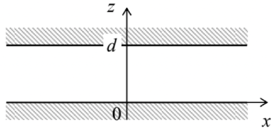Fig. 2.6. The plane capacitor as the system for the simplest illustration of the boundary problem (35) and its solution.

In these coordinates, the Laplace operator is just the sum of 3 second derivatives.²⁰ It is evident that due to the problem’s translational symmetry in the [x, y] plane, deep inside the gap (i.e. at the lateral distance from the edges much larger than \(\ d\)) the electrostatic potential may only depend on the coordinate normal to the gap surfaces: \(\ \phi(\mathbf{r})=\phi(z)\). For such a function, the derivatives over x and y vanish, and the boundary problem (35) is reduced to a very simple ordinary differential equation

\[\ \frac{d^{2} \phi}{d z^{2}}(z)=0,\tag{2.37}\]

with boundary conditions

\[\ \phi(0)=0, \quad \phi(d)=V.\tag{2.38}\]

(For the sake of notation simplicity, I have used the discretion of adding a constant to the potential, to make one of the potentials vanish, and also the definition (25) of the voltage \(\ V\).) The general solution of Eq. (37) is a linear function: \(\ \phi(z)=c_{1} z+c_{2}\), whose constant coefficients \(\ c_{1,2}\) may be readily found from the boundary conditions (38). The final solution is

\[\ \phi=V \frac{z}{d}.\tag{2.39}\]

From here the only nonzero component of the electric field is

\[\ E_{z}=-\frac{d \phi}{d z}=-\frac{V}{d},\tag{2.40}\]

and the surface charge of the capacitor plates is

\[\ \sigma=\varepsilon_{0} E_{n}=\mp \varepsilon_{0} E_{z}=\pm \varepsilon_{0} \frac{V}{d},\tag{2.41}\]

where the upper and lower signs correspond to the upper and lower plate, respectively. Since \(\ \sigma\) does not depend on x and y, we can get the full charges \(\ Q_{1}=-Q_{2} \equiv Q\) of the surfaces by its multiplication by the gap area \(\ A\), giving us again the already obtained result (28) for the mutual capacitance \(\ C \equiv Q / V\). I believe that this calculation, though very easy, may serve as a good illustration of the boundary problem solution approach, which will be used below for more complex cases.

(ii) Coaxial-cable capacitor. Coaxial cable is a system of two round cylindrical, coaxial conductors, with the cross-section shown in Fig. 7.

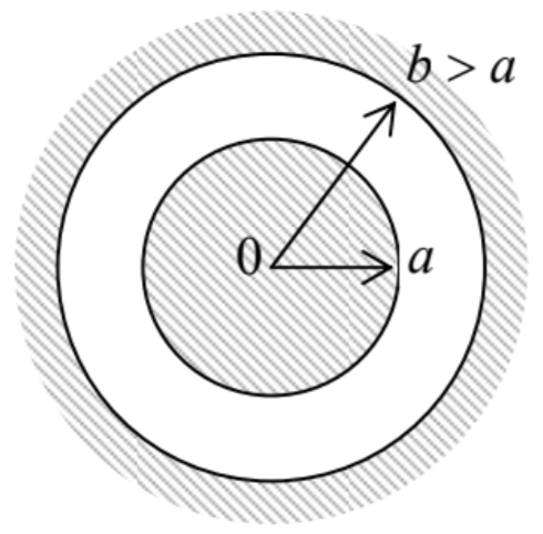Fig. 2.7. The cross-section of a coaxial cable.

Evidently, in this case the cylindrical coordinates \(\ \{\rho, \varphi, z\}\), with the z-axis coinciding with the common axis of the cylinders, are most convenient. Due to the axial symmetry of the problem, in these coordinates \(\ \mathbf{E}(\mathbf{r})=\mathbf{n}_{\rho} E(\rho)\), \(\ \phi(\mathbf{r})=\phi(\rho)\), so that in the general expression for the Laplace operator²¹ we can take \(\ \partial / \partial \varphi=\partial / \partial z=0\). As a result, only the radial term of the operator survives, and the boundary problem (35) takes the form

\[\ \frac{1}{\rho} \frac{d}{d \rho}\left(\rho \frac{d \phi}{d \rho}\right)=0, \quad \phi(a)=V, \quad \phi(b)=0.\tag{2.42}\]

The sequential double integration of this ordinary linear differential equation is elementary (and similar to that of the Poisson equation in spherical coordinates, carried out in Sec. 1.3), giving

\[\ \rho \frac{d \phi}{d \rho}=c_{1}, \quad \phi(\rho)=c_{1} \int_{a}^{\rho} \frac{d \rho^{\prime \prime}}{\rho^{\prime \prime}}+c_{2}=c_{1} \ln \frac{\rho}{a}+c_{2}.\tag{2.43}\]

The constants \(\ \mathcal{C}_{1,2}\) may be found using boundary conditions (42):

\[\ c_{2}=V, \quad c_{1} \ln \frac{b}{a}+c_{2}=0,\tag{2.44}\]

giving \(\ c_{1}=-V / \ln (b / a)\), so that solution (43) takes the following form:

\[\ \phi(\rho)=V\left[1-\frac{\ln (\rho / a)}{\ln (b / a)}\right].\tag{2.45}\]

Next, for our axial symmetry, the general expression for the gradient of a scalar function is reduced to its radial derivative, so that

\[\ E(\rho) \equiv-\frac{d \phi(\rho)}{d \rho}=\frac{V}{\rho \ln (b / a)}.\tag{2.46}\]

This expression, plugged into Eq. (2), allows us to find the density of conductors’ surface charge. For example, for the inner electrode

\[\ \sigma_{a}=\varepsilon_{0} E(a)=\frac{\varepsilon_{0} V}{a \ln (b / a)},\tag{2.47}\]

so that its full charge (per unit length of the system) is

\[\ \frac{Q}{l}=2 \pi a \sigma_{a}=\frac{2 \pi \varepsilon_{0} V}{\ln (b / a)}.\tag{2.48}\]

(It is straightforward to check that the charge of the outer electrode is equal and opposite.) Hence, by the definition of the mutual capacitance, its value per unit length is

C: Coaxial cable

\[\ \frac{C}{l} \equiv \frac{Q}{l V}=\frac{2 \pi \varepsilon_{0}}{\ln (b / a)}.\tag{2.49}\]

This expression shows that the total capacitance \(\ C\) is proportional to the systems length \(\ l\) (if \(\ l \gg a,b\)), while being only logarithmically dependent on is the dimensions of its cross-section. Since the logarithm of a very large argument is an extremely slow function (sometimes called a quasi-constant), if the external conductor is made very large \(\ (b \gg a)\), the capacitance diverges, but very weakly. Such logarithmic divergence may be cut by any minuscule additional effect, for example by the finite length \(\ l\) of the system. This allows one to get a very useful estimate of the self-capacitance of a single round wire of radius \(\ a\):

\[\ C \approx \frac{2 \pi \varepsilon_{0} l}{\ln (l / a)}, \quad \text { for } l>>a.\tag{2.50}\]

On the other hand, if the gap \(\ d\) between the conductors is very narrow: \(\ d \equiv b-a<<a\), then \(\ \ln (b / a) \equiv \ln (1+d / a)\) may be approximated as \(\ d / a\), and Eq. (49) is reduced to \(\ C \approx 2 \pi \varepsilon_{0} al / d\), i.e. to Eq. (28) for the plane capacitor, of the appropriate area \(\ A=2 \pi al\).

(iii) Spherical capacitor. This is a system of two conductors, with the central cross-section similar to that of the coaxial cable (Fig. 7), but now with the spherical rather than axial symmetry. This symmetry implies that we would be better off using spherical coordinates, so that the potential \(\ \phi\) depends only on one of them: the distance \(\ r\) from the common center of the conductors: \(\ \phi(\mathbf{r})=\phi(r)\). As we already know from Sec. 1.3, in this case the general expression for the Laplace operator is reduced to its first (radial) term, so that the Laplace equation takes the simple form (1.47). Moreover, we have already found the general solution to this equation – see Eq. (1.50):

\[\ \phi(r)=\frac{c_{1}}{r}+c_{2},\tag{2.51}\]

Now acting exactly as above, i.e. determining the (only essential) constant \(\ c_{1}\) from the boundary condition \(\ \phi(a)-\phi(b)=V\), we get

\[\ c_{1}=V\left(\frac{1}{a}-\frac{1}{b}\right)^{-1}, \quad \text { so that } \phi(r)=\frac{V}{r}\left(\frac{1}{a}-\frac{1}{b}\right)^{-1}+c_{2}.\tag{2.52}\]

Next, we can use the spherical symmetry to find the electric field, \(\ \mathbf{E}(\mathbf{r})=\mathbf{n}_{r} E(r)\), with

\[\ E(r)=-\frac{d \phi}{d r}=\frac{V}{r^{2}}\left(\frac{1}{a}-\frac{1}{b}\right)^{-1},\tag{2.53}\]

and hence its values on conductors’ surfaces, and then the surface charge density \(\ \sigma\) from Eq. (3). For example, for the inner conductor’s surface,

\[\ \sigma_{a}=\varepsilon_{0} E(a)=\varepsilon_{0} \frac{V}{a^{2}}\left(\frac{1}{a}-\frac{1}{b}\right)^{-1},\tag{2.54}\]

so that, finally, for the full charge of that conductor we get the following result:

\[\ Q=4 \pi a^{2} \sigma=4 \pi \varepsilon_{0}\left(\frac{1}{a}-\frac{1}{b}\right)^{-1} V.\tag{2.55}\]

(Again, the charge of the outer conductor is equal and opposite.) Now we can use the definition (26) of the mutual capacitance to get the final result

C: Spherical capacitor

\[\ C \equiv \frac{Q}{V}=4 \pi \varepsilon_{0}\left(\frac{1}{a}-\frac{1}{b}\right)^{-1} \equiv 4 \pi \varepsilon_{0} \frac{a b}{b-a}.\tag{2.56}\]

For \(\ b \gg a\), this result coincides with Eq. (17) for the self-capacitance of the inner conductor. On the other hand, if the gap \(\ d\) between two conductors is narrow, \(\ d \equiv b-a<<a\), then

\[\ C=4 \pi \varepsilon_{0} \frac{a(a+d)}{d} \approx 4 \pi \varepsilon_{0} \frac{a^{2}}{d},\tag{2.57}\]

i.e. the capacitance approaches that of the planar capacitor of the area \(\ A=4 \pi a^{2}\) – as it should.

All this seems (and indeed is) very straightforward, but let us contemplate what was the reason for such easy successes. In each of the cases (i)-(iii) we have managed to find such coordinates that both the Laplace equation and the boundary conditions involved only one of them. The necessary condition for the former fact is that the coordinates are orthogonal. This means that the three vector components of the local differential dr, due to small variations of the new coordinates (say, \(\ dr\), \(\ d \theta\), and \(\ d \varphi\) for the spherical coordinates), are mutually perpendicular.

---

Reference

²⁰ See, e.g. MA Eq. (9.1).

²¹ See, e.g., MA Eq. (10.3).