
2.8: Variable Separation – Cartesian Coordinates
- Page ID
- 56973

The general approach of the methods discussed in the last two sections was to satisfy the Laplace equation by a function of a single variable that also satisfies the boundary conditions. Unfortunately, in many cases this cannot be done – at least, using sufficiently simple functions. In this case, a very powerful method called the variable separation,33 may work, typically producing “semi-analytical” results in the form of series (infinite sums) of either elementary or well-studied special functions. Its main idea is to look for the solution of the boundary problem (35) as the sum of partial solutions,
\[\ \phi=\sum_{k} c_{k} \phi_{k},\tag{2.84}\]
where each function \(\ \phi_{k}\) satisfies the Laplace equation, and then select the set of coefficients \(\ c_{k}\) to satisfy the boundary conditions. More specifically, in the variable separation method, the partial solutions \(\ \phi_{k}\) are looked for in the form of a product of functions, each depending on just one spatial coordinate.
Let us discuss this approach on the classical example of a rectangular box with conducting walls (Fig. 13), with the same potential (that I will take for zero) at all its sidewalls and the lower lid, but a different potential \(\ V\) at the top lid \(\ (z=c)\). Moreover, to demonstrate the power of the variable separation method, let us carry out all the calculations for a more general case when the top lid’s potential is an arbitrary 2D function \(\ V(x, y)\).34
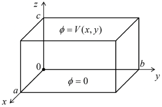
For this geometry, it is natural to use the Cartesian coordinates \(\ \{x, y, z\}\), representing each of the partial solutions in Eq. (84) as the following product
\[\ \phi_{k}=X(x) Y(y) Z(z).\tag{2.85}\]
Plugging it into the Laplace equation expressed in the Cartesian coordinates,
\[\ \frac{\partial^{2} \phi_{k}}{\partial x^{2}}+\frac{\partial^{2} \phi_{k}}{\partial y^{2}}+\frac{\partial^{2} \phi_{k}}{\partial z^{2}}=0,\tag{2.86}\]
and dividing the result by XYZ, we get
\[\ \frac{1}{X} \frac{d^{2} X}{d x^{2}}+\frac{1}{Y} \frac{d^{2} Y}{d y^{2}}+\frac{1}{Z} \frac{d^{2} Z}{d z^{2}}=0.\tag{2.87}\]
Here comes the punch line of the variable separation method: since the first term of this sum may depend only on \(\ x\), the second one only of y, etc., Eq. (87) may be satisfied everywhere in the volume only if each of these terms equals a constant. In a minute we will see that for our current problem (Fig. 13), these constant \(\ x\)- and \(\ y\)-terms have to be negative; hence let us denote these variable separation constants as \(\ \left(-\alpha^{2}\right)\) and \(\ \left(-\beta^{2}\right)\), respectively. Now Eq. (87) shows that the constant z-term has to be positive; denoting it as \(\ \gamma^{2}\) we get the following relation:
\[\ \alpha^{2}+\beta^{2}=\gamma^{2}.\tag{2.88}\]
Now the variables are separated in the sense that for the functions \(\ X(x)\), \(\ Y(y)\), and \(\ Z(z)\) we have got separate ordinary differential equations,
\[\ \frac{d^{2} X}{d x^{2}}+\alpha^{2} X=0, \quad \frac{d^{2} Y}{d y^{2}}+\beta^{2} Y=0, \quad \frac{d^{2} Z}{d z^{2}}-\gamma^{2} Z=0,\tag{2.89}\]
which are related only by Eq. (88) for their constant parameters.
Let us start from the equation for the function \(\ X(x)\). Its general solution is the sum of functions \(\ \sin \alpha x\) and \(\ \cos \alpha x\), multiplied by arbitrary coefficients. Let us select these coefficients to satisfy our boundary conditions. First, since \(\ \phi \propto X\) should vanish at the back vertical wall of the box (i.e., with the
coordinate origin choice shown in Fig. 13, at \(\ x = 0\) for any \(\ y\) and \(\ z\)), the coefficient at \(\ \cos \alpha x\) should be zero. The remaining coefficient (at \(\ \sin \alpha x\)) may be included in the general factor \(\ c_{k}\) in Eq. (84), so that we may take \(\ X\) in the form
\[\ X=\sin \alpha x.\tag{2.90}\]
This solution satisfies the boundary condition at the opposite wall \(\ (x=a)\) only if the product \(\ \alpha a\) is a multiple of \(\ \pi\), i.e. if \(\ \alpha\) is equal to any of the following numbers (commonly called eigenvalues):35
\[\ \alpha_{n}=\frac{\pi}{a} n, \quad \text { with } n=1,2, \ldots\tag{2.91}\]
(Terms with negative values of \(\ n\) would not be linearly-independent from those with positive \(\ n\), and may be dropped from the sum (84). The value \(\ n = 0\) is formally possible, but would give \(\ X = 0\), i.e. \(\ \phi_{k}=0\), at any \(\ x\), i.e. no contribution to sum (84), so it may be dropped as well.) Now we see that we indeed had to take \(\ \alpha\) real (i.e. \(\ \alpha^{2}\) positive) – otherwise, instead of the oscillating function (90) we would have a sum of two exponential functions, which cannot equal zero at two independent points of the \(\ x\)-axis.
Since the equation (89) for function \(\ Y(y)\) is similar to that for \(\ X(x)\), and the boundary conditions on the walls perpendicular to axis \(\ y\) (\(\ y = 0\) and \(\ y = b\)) are similar to those for \(\ x\)-walls, the absolutely similar reasoning gives
\[\ Y=\sin \beta y, \quad \beta_{m}=\frac{\pi}{b} m, \quad \text { with } m=1,2, \ldots,\tag{2.92}\]
where the integer \(\ m\) may be selected independently of \(\ n\). Now we see that according to Eq. (88), the separation constant \(\ \gamma\) depends on two integers \(\ n\) and \(\ m\), so that the relationship may be rewritten as
\[\ \gamma_{n m}=\left[\alpha_{n}^{2}+\beta_{m}^{2}\right]^{1 / 2}=\pi\left[\left(\frac{n}{a}\right)^{2}+\left(\frac{m}{b}\right)^{2}\right]^{1 / 2}.\tag{2.93}\]
The corresponding solution of the differential equation for \(\ Z\) may be represented as a linear combination of two exponents \(\ \exp \left\{\pm \gamma_{n m} z\right\}\), or alternatively of two hyperbolic functions, \(\ \sinh \gamma_{n m} z\) and \(\ \cosh \gamma_{n m} z\), with arbitrary coefficients. At our choice of coordinate origin, the latter option is preferable, because \(\ \cosh \gamma_{n m} z\) cannot satisfy the zero boundary condition at the bottom lid of the box \(\ (z = 0)\). Hence we may take \(\ Z\) in the form
\[\ Z=\sinh \gamma_{n m} z,\tag{2.94}\]
which automatically satisfies that condition.
Now it is the right time to merge Eqs. (84)-(85) and (90)-(94), replacing the temporary index \(\ k\) with the full set of possible eigenvalues, in our current case of two integer indices \(\ n\) and \(\ m\):
Variable separation in Cartesian coordinates (example)
\[\ \phi(x, y, z)=\sum_{n, m=1}^{\infty} c_{n m} \sin \frac{\pi n x}{a} \sin \frac{\pi m y}{b} \sinh \gamma_{n m} z,\tag{2.95}\]
where \(\ \gamma_{n m}\) is given by Eq. (93). This solution satisfies not only the Laplace equation, but also the boundary conditions on all walls of the box, besides the top lid, for arbitrary coefficients \(\ c_{n m}\). The only job left is to choose these coefficients from the top-lid requirement:
\[\ \phi(x, y, c) \equiv \sum_{n, m=1}^{\infty} c_{n m} \sin \frac{\pi n x}{a} \sin \frac{\pi m y}{b} \sinh \gamma_{n m} c=V(x, y).\tag{2.96}\]
It may look bad to have just one equation for the infinite set of coefficients \(\ c_{n m}\). However, the decisive help comes from the fact that the functions of x and y that participate in Eq. (96), form full, orthogonal sets of 1D functions. The last term means that the integrals of the products of the functions with different integer indices over the region of interest equal zero. Indeed, a direct integration gives
\[\ \int_{0}^{a} \sin \frac{\pi n x}{a} \sin \frac{\pi n^{\prime} x}{a} d x=\frac{a}{2} \delta_{n n^{\prime}},\tag{2.97}\]
where \(\ \delta_{n n}\), is the Kronecker symbol, and similarly for \(\ y\) (with the evident replacements \(\ a \rightarrow b\), and \(\ n \rightarrow m\)). Hence, a fruitful way to proceed is to multiply both sides of Eq. (96) by the product of the basis functions, with arbitrary indices \(\ n^\prime\) and \(\ m^\prime\), and integrate the result over \(\ x\) and \(\ y\):
\[\ \sum_{n, m=1}^{\infty} c_{n m} \sinh \gamma_{n m} c \int_{0}^{a} \sin \frac{\pi n x}{a} \sin \frac{\pi n^{\prime} x}{a} d x \int_{0}^{b} \sin \frac{\pi m y}{b} \sin \frac{\pi m^{\prime} y}{b} d y=\int_{0}^{a} d x \int_{0}^{b} d y V(x, y) \sin \frac{\pi n^{\prime} x}{a} \sin \frac{\pi m^{\prime} y}{b}.\tag{2.98}\]
Due to Eq. (97), all terms on the left-hand side of the last equation, besides those with \(\ n=n^{\prime}\) and \(\ m=m^{\prime}\), vanish, and (replacing \(\ n^{\prime}\) with \(\ n\), and \(\ m^{\prime}\) with \(\ m\), for notation brevity) we finally get
\[\ c_{n m}=\frac{4}{a b \sinh \gamma_{n m} c} \int_{0}^{a} d x \int_{0}^{b} d y V(x, y) \sin \frac{\pi n x}{a} \sin \frac{\pi m y}{b}.\tag{2.99}\]
The relations (93), (95), and (99) give the complete solution of the posed boundary problem; we can see both good and bad news here. The first bit of bad news is that in the general case we still need to work out the integrals (99) – formally, the infinite number of them. In some cases, it is possible to do this analytically, in one shot. For example, if the top lid in our problem is a single conductor, i.e. has a constant potential \(\ V_{0}\), we may take \(\ V(x, y)=V_{0}=\mathrm{const}\), and both 1D integrations are elementary; for example
\[\ \int_{0}^{a} \sin \frac{\pi n x}{a} d x=\frac{2 a}{\pi n} \times \begin{cases}1, & \text { for } n \text { odd, } \\ 0, & \text { for } n \text { even, }\end{cases}\tag{2.100}\]
and similarly for the integral over \(\ y\), so that
\[\ c_{n m}=\frac{16 V_{0}}{\pi^{2} n m \sinh \gamma_{n m} c} \times \begin{cases}1, & \text { if both } n \text { and } m \text { are odd, } \\ 0, & \text { otherwise. }\end{cases}\tag{2.101}\]
The second bad news is that even on such a happy occasion, we still have to sum up the series (95), so that our result may only be called analytical with some reservations, because in most cases we need a computer to get the final numbers or plots.
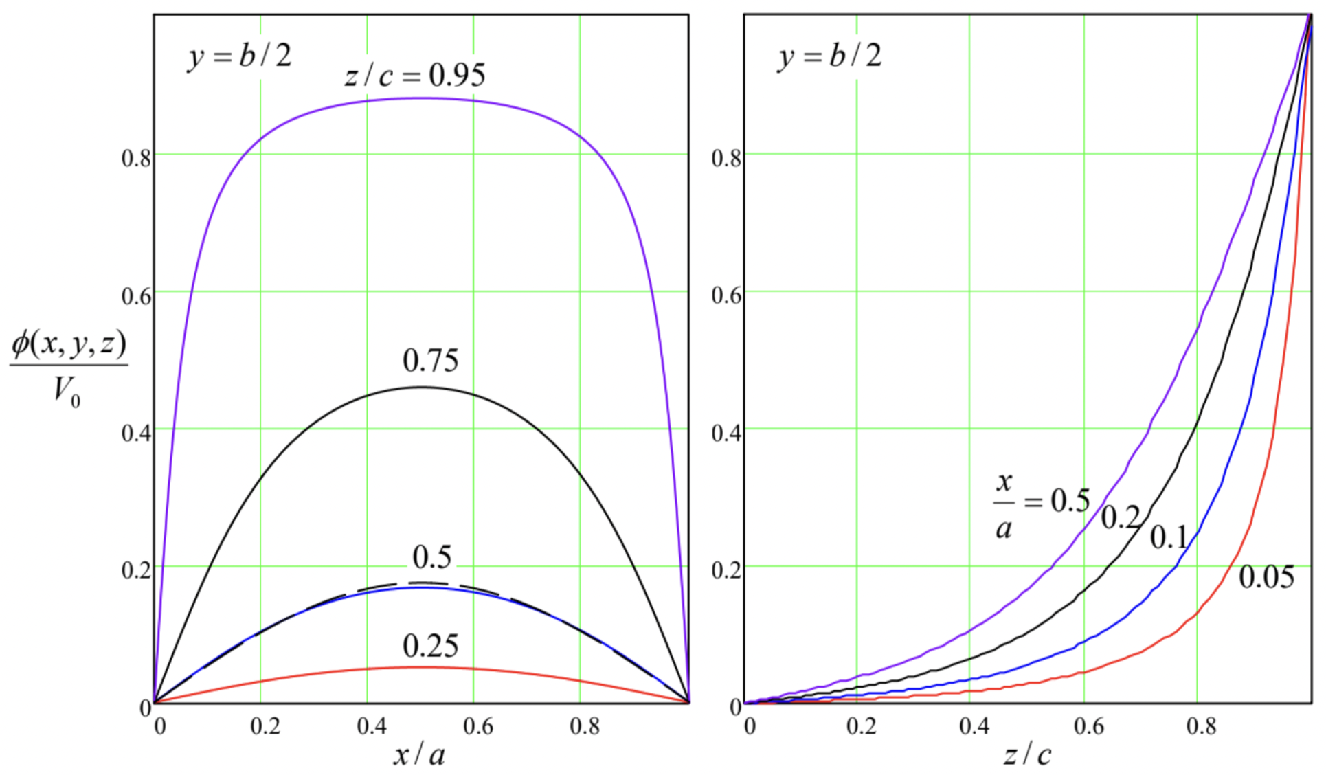
Now the first good news. Computers are very efficient for both operations (95) and (99), i.e. for the summation and integration. (As was discussed in Sec. 1.2, random errors are averaged out at these operations.) As an example, Fig. 14 shows the plots of the electrostatic potential in a cubic box \(\ (a = b = c)\), with an equipotential top lid \(\ \left(V=V_{0}=\mathrm{cons} \mathrm{t}\right)\), obtained by a numerical summation of the series (95), using the analytical expression (101). The remarkable feature of this calculation is a very fast convergence of the series; for the middle cross-section of the cubic box \(\ (z / c=0.5)\), already the first term (with \(\ n = m = 1\)) gives an accuracy about 6%, while the sum of four leading terms (with \(\ n, m = 1, 3\)) reduces the error to just 0.2%. (For a longer box, \(\ c > a, b\), the convergence is even faster – see the discussion below.) Only very close to the corners between the top lid and the sidewalls, where the potential changes rapidly, several more terms are necessary to get a reasonable accuracy.
The related piece of good news is that our “semi-analytical” result allows its ultimate limits to be explored analytically. For example, Eq. (93) shows that for a very flat box (with \(\ c<<a, b\)), \(\ \gamma_{n, m} z \leq \gamma_{n, m} c<<1\) at least for the lowest terms of series (95), with \(\ n, m<<c / a, c / b\). In this case, the sinh functions in
Eqs. (96) and (99) may be well approximated with their arguments, and their ratio by \(\ z / c\). So if we limit the summation to these terms, Eq. (95) gives a very simple result
\[\ \phi(x, y) \approx \frac{z}{c} V(x, y),\tag{2.102}\]
which means that each segment of the flat box behaves just as a plane capacitor. Only near the sidewalls, the higher terms in the series (95) are important, producing some deviations from Eq. (102). (For the general problem with an arbitrary function V(x,y), this is also true at all regions where this function changes sharply.)
In the opposite limit \(\ (a, b<<c)\), Eq. (93) shows that, in contrast, \(\ \gamma_{n, m} c \quad>>1\) for all \(\ n\) and \(\ m\). Moreover, the ratio \(\ \sinh \gamma_{n, m} z / \sinh \gamma_{n, m} c\) drops sharply if either \(\ n\) or \(\ m\) is increased, provided that \(\ z\) is not too close to \(\ c\). Hence in this case a very good approximation may be obtained by keeping just the leading term, with \(\ n = m = 1\), in Eq. (95), so that the challenge of summation disappears. (As was discussed above, this approximation works reasonably well even for a cubic box.) In particular, for the constant potential of the upper lid, we can use Eq. (101) and the exponential asymptotic for both sinh functions, to get a very simple formula:
\[\ \phi=\frac{16}{\pi^{2}} \sin \frac{\pi x}{a} \sin \frac{\pi y}{b} \exp \left\{-\pi \frac{\left(a^{2}+b^{2}\right)^{1 / 2}}{a b}(c-z)\right\}.\tag{2.103}\]
These results may be readily generalized to some other problems. For example, if all walls of the box shown in Fig. 13 have an arbitrary potential distribution, we may use the linear superposition principle to represent the electrostatic potential distribution as the sum of six partial solutions of the type of Eq. (95), each with one wall biased by the corresponding voltage, and all other grounded \(\ (\phi=0)\).
To summarize, the results given by the variable separation method in the Cartesian coordinates are closer to what we could call a genuinely analytical solution than to purely numerical solutions. Now, let us explore the issues that arise when this method is applied in other orthogonal coordinate systems.
Reference
33 Again, this method was already discussed in CM Sec. 6.5 and then used also in Secs. 6.6 and 8.4 of that course. However, the method is so important that I need to repeat its discussion in this part of my series, for the benefit of the readers who have skipped the Classical Mechanics course for whatever reason.
34 Such voltage distributions may be implemented in practice using the so-called mosaic electrodes consisting of many electrically-insulated and individually-biased panels.
35 Note that according to Eqs. (91)-(92), as the spatial dimensions a and b of the system are increased, the distances between the adjacent eigenvalues tend to zero. This fact implies that for spatially-infinite systems, the eigenvalue spectra are continuous, so that the sums of the type (84) become integrals. A few problems of this type are provided in Sec. 9 for the reader’s exercise.